Code Reproducibility

from graspologic.simulations import er_np
import numpy as np

p = 0.3
A = er_np(n=50, p=p)

from graspologic.models import EREstimator

model = EREstimator(directed=False, loops=False)
model.fit(A)
# obtain the estimate from the fit model
phat = model.p_

print("Difference between phat and p: {:.3f}".format(phat - p))

Difference between phat and p: -0.001

from graspologic.simulations import sbm

n = [50, 50]
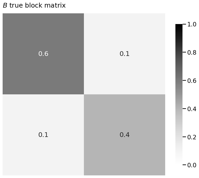
B = np.array([[0.6, 0.1], 
              [0.1, 0.4]])

A, z = sbm(n=n, p=B, return_labels=True)

from graspologic.models import SBMEstimator
from graphbook_code import heatmap

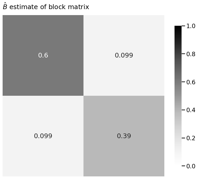
model = SBMEstimator(directed=False, loops=False)
model.fit(A, y=z)
Bhat = model.block_p_

# plot the block matrix vs estimate
heatmap(B, title="$B$ true block matrix", vmin=0, vmax=1, annot=True)
heatmap(Bhat, title=r"$\hat B$ estimate of block matrix", vmin=0, vmax=1, annot=True)
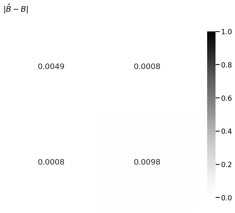
heatmap(np.abs(Bhat - B), title=r"$|\hat B - B|$", vmin=0, vmax=1, annot=True)

<Axes: title={'left': '$|\\hat B - B|$'}>

from graspologic.simulations import sbm
from graphbook_code import generate_sbm_pmtx, lpm_from_sbm
import numpy as np

n = 100
# construct the block matrix B as described above
B = np.array([[0.6, 0.1], 
              [0.1, 0.4]])

# sample a graph from SBM_{100}(tau, B)
np.random.seed(0)
A, zs = sbm(n=[n//2, n//2], p=B, return_labels=True)

X = lpm_from_sbm(zs, B)
P = generate_sbm_pmtx(zs, B)

from graspologic.embed import AdjacencySpectralEmbed as ase

d = 2  # the latent dimensionality
# estimate the latent position matrix with ase
Xhat = ase(n_components=d, svd_seed=0).fit_transform(A)

Phat = Xhat @ Xhat.transpose()

vtx_perm = np.random.choice(n, size=n, replace=False)

# reorder the adjacency matrix
Aperm = A[tuple([vtx_perm])] [:,vtx_perm]
# reorder the community assignment vector
zperm = np.array(zs)[vtx_perm]

# compute the estimated latent positions using the
# permuted adjacency matrix
Xhat_perm = ase(n_components=2).fit_transform(Aperm)

from graspologic.plot import pairplot

pairplot(Xhat, title=r"Pairs plot of $\hat X$")

/opt/hostedtoolcache/Python/3.12.5/x64/lib/python3.12/site-packages/seaborn/axisgrid.py:1513: UserWarning: Ignoring `palette` because no `hue` variable has been assigned.
  func(x=vector, **plot_kwargs)
/opt/hostedtoolcache/Python/3.12.5/x64/lib/python3.12/site-packages/seaborn/axisgrid.py:1513: UserWarning: Ignoring `palette` because no `hue` variable has been assigned.
  func(x=vector, **plot_kwargs)
/opt/hostedtoolcache/Python/3.12.5/x64/lib/python3.12/site-packages/seaborn/axisgrid.py:1615: UserWarning: Ignoring `palette` because no `hue` variable has been assigned.
  func(x=x, y=y, **kwargs)
/opt/hostedtoolcache/Python/3.12.5/x64/lib/python3.12/site-packages/seaborn/axisgrid.py:1615: UserWarning: Ignoring `palette` because no `hue` variable has been assigned.
  func(x=x, y=y, **kwargs)

<seaborn.axisgrid.PairGrid at 0x7f17ed804860>

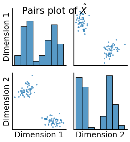
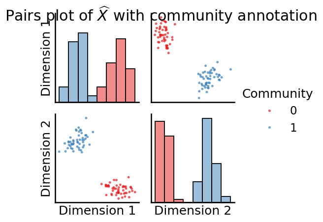
fig = pairplot(Xhat_perm, labels=zperm, legend_name = "Community",
             title=r"Pairs plot of $\widehat X$ with community annotation",
             diag_kind="hist")

from scipy.spatial import distance_matrix

D = distance_matrix(Xhat, Xhat)

import numpy as np
from graphbook_code import dcsbm

nk = 150
z = np.repeat([1,2], nk)
B = np.array([[0.6, 0.2], [0.2, 0.4]])
theta = np.tile(6**np.linspace(0, -1, nk), 2)
np.random.seed(0)
A, P = dcsbm(z, theta, B, return_prob=True)

from graspologic.embed import AdjacencySpectralEmbed as ase
from scipy.spatial import distance_matrix

d = 2  # the latent dimensionality
# estimate the latent position matrix with ase
Xhat = ase(n_components=d, svd_seed=0).fit_transform(A)
# compute the distance matrix
D = distance_matrix(Xhat, Xhat)

Xhat_rescaled = Xhat / theta[:,None]
D_rescaled = distance_matrix(Xhat_rescaled, Xhat_rescaled)

from graspologic.embed import LaplacianSpectralEmbed as lse

d = 2  # embed into two dimensions
Xhat_lapl = lse(n_components=d, svd_seed=0).fit_transform(A)
D_lapl = distance_matrix(Xhat_lapl, Xhat_lapl)

import seaborn as sns
import pandas as pd

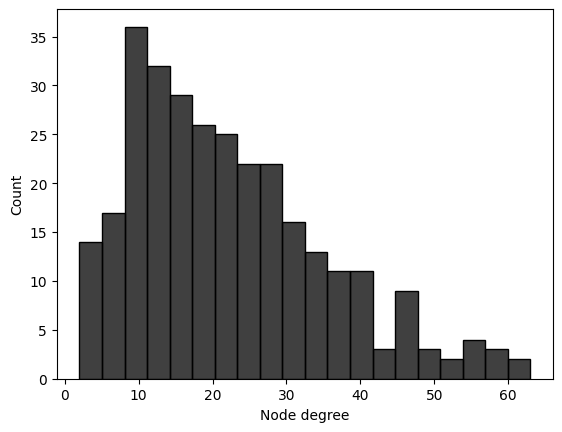
# compute the degrees for each node, using the
# row-sums of the network
degrees = A.sum(axis = 0)

# plot the degree histogram
df = pd.DataFrame({"Node degree" : degrees, "Community": z})
sns.histplot(data=df, x="Node degree", bins=20, color="black")

<Axes: xlabel='Node degree', ylabel='Count'>

Asbm = sbm([nk, nk], B)

# row-sums of the network
degrees_sbm = Asbm.sum(axis = 0)

from graspologic.simulations import sbm
import numpy as np
from sklearn.preprocessing import LabelEncoder

n = 100  # the number of nodes
M = 8  # the total number of networks
# human brains have homophilic block structure
Bhuman = np.array([[0.2, 0.02], [0.02, 0.2]])
# alien brains have a core-periphery block structure
Balien = np.array([[0.4, 0.2], [0.2, 0.1]])

# set seed for reproducibility
np.random.seed(0)

# generate 4 human and 4 alien brain networks
A_humans = [sbm([n // 2, n // 2], Bhuman) for i in range(M // 2)]
A_aliens = [sbm([n // 2, n // 2], Balien) for i in range(M // 2)]
# concatenate list of human and alien networks
networks = A_humans + A_aliens

# 1 = left hemisphere, 2 = right hemisphere for node communities
le = LabelEncoder()
labels = np.repeat(["L", "R"], n//2)
zs = le.fit_transform(labels) + 1

from graspologic.embed import AdjacencySpectralEmbed as ase

# embed the first network
Xhat = ase(n_components=2, svd_seed=0).fit_transform(A_humans[0])

# a rotation by 90 degrees
W = np.array([[0, -1], [1, 0]])
Yhat = Xhat @ W

# check that probability matrix is the same
np.allclose(Yhat @ Yhat.transpose(), Xhat @ Xhat.transpose())
# returns True

True

# a reflection across first latent dimension
Wp = np.array([[-1, 0], [0, 1]])
Zhat = Xhat @ Wp
# check that the probability matrix is the same
# check that probability matrix is the same
np.allclose(Zhat @ Zhat.transpose(), Xhat @ Xhat.transpose())
# returns True

True

# embed the third human network
Xhat3 = ase(n_components=2, svd_seed=0).fit_transform(A_humans[3])

# embed the first alien network
Xhat_alien = ase(n_components=2, svd_seed=0).fit_transform(A_aliens[0])

# compute frob norm between first human and third human net
# estimated latent positions
dist_firsthum_thirdhum = np.linalg.norm(Xhat - Xhat3, ord="fro")
print("Frob. norm(first human, third human) = {:3f}".format(dist_firsthum_thirdhum))
# Frob. norm(first human, third human) = 8.798482

# compute frob norm between first human and first alien net
# estimated latent positions
dist_firsthum_alien = np.linalg.norm(Xhat - Xhat_alien, ord="fro")
print("Frob. norm(first human, alien) = {:3f}".format(dist_firsthum_alien))
# Frob. norm(first human, alien) = 5.991560

Frob. norm(first human, third human) = 6.302736
Frob. norm(first human, alien) = 5.182462

from graspologic.embed import MultipleASE as mase

# Use mase to embed everything
mase = mase(n_components=2, svd_seed=0)
# fit_transform on the human and alien networks simultaneously
latents_mase = mase.fit_transform(networks)

from graspologic.embed import AdjacencySpectralEmbed as ase

dhat = int(np.ceil(np.log2(n)))
# spectrally embed each network into ceil(log2(n)) dimensions with ASE
separate_embeddings = [ase(n_components=dhat, svd_seed=0).fit_transform(network) for network in networks]

# Concatenate the embeddings horizontally into a single n x Md matrix
joint_matrix = np.hstack(separate_embeddings)

def unscaled_embed(X, d, seed=0):
    np.random.seed(seed)
    U, s, Vt = np.linalg.svd(X)
    return U[:,0:d]

Shat = unscaled_embed(joint_matrix, 2)

# stack the networks into a numpy array
As_ar = np.asarray(networks)
# compute the scores
scores = Shat.T @ As_ar @ Shat

from graphbook_code import generate_sbm_pmtx

Phum = generate_sbm_pmtx(zs, Bhuman)
Palien = generate_sbm_pmtx(zs, Balien)
Pests = Shat @ scores @ Shat.T

from graspologic.embed import MultipleASE as mase

d = 2
mase_embedder = mase(n_components=d)
# obtain an estimate of the shared latent positions
Shat = mase_embedder.fit_transform(networks)
# obtain an estimate of the scores
Rhat_hum1 = mase_embedder.scores_[0]
# obtain an estimate of the probability matrix for the first human
Phat_hum1 = Shat @ mase_embedder.scores_[0] @ Shat.T

omni_ex = np.block(
    [[networks[0], (networks[0]+networks[1])/2],
     [(networks[1]+networks[0])/2, networks[1]]]
)

from graspologic.embed.omni import _get_omni_matrix
omni_mtx = _get_omni_matrix(networks)

from graspologic.embed import AdjacencySpectralEmbed as ase

dhat = int(np.ceil(np.log2(n)))
Xhat_omni = ase(n_components=dhat, svd_seed=0).fit_transform(omni_mtx)

M = len(networks)
n = len(networks[0])

# obtain an M x n x d tensor
Xhat_tensor = Xhat_omni.reshape(M, n, -1)
# the estimated latent positions for the first network
Xhat_human1 = Xhat_tensor[0,:,:]

from graspologic.embed import OmnibusEmbed as omni

# obtain a tensor of the estimated latent positions
Xhat_tensor = omni(n_components=int(np.log2(n)), svd_seed=0).fit_transform(networks)
# obtain the estimated latent positions for the first human
# network
Xhat_human1 = Xhat_tensor[0,:,:]

Phat_hum1 = Xhat_human1 @ Xhat_human1.T

from graspologic.simulations import sbm
import numpy as np

n = 200  # total number of nodes
# first two communities are the ``core'' pages for statistics
# and computer science, and second two are the ``peripheral'' pages
# for statistics and computer science.
B = np.array([[.4, .3, .05, .05],
              [.3, .4, .05, .05],
              [.05, .05, .05, .02],
              [.05, .05, .02, .05]])

# make the stochastic block model
np.random.seed(0)
A, labels = sbm([n // 4, n // 4, n // 4, n // 4], B, return_labels=True)
# generate labels for core/periphery
co_per_labels = np.repeat(["Core", "Periphery"], repeats=n//2)
# generate labels for statistics/CS.
st_cs_labels = np.repeat(["Stat", "CS", "Stat", "CS"], repeats=n//4)

trial = []
for label in st_cs_labels:
    if "Stat" in label:
        # if the page is a statistics page, there is a 50% chance
        # of citing each of the scholars
        trial.append(np.random.binomial(1, 0.5, size=20))
    else:
        # if the page is a CS page, there is a 5% chance of citing
        # each of the scholars
        trial.append(np.random.binomial(1, 0.05, size=20))
Y = np.vstack(trial)

def embed(X, d=2, seed=0):
    """
    A function to embed a matrix.
    """
    np.random.seed(seed)
    Lambda, V = np.linalg.eig(X)
    return V[:, 0:d] @ np.diag(np.sqrt(np.abs(Lambda[0:d])))

def pca(X, d=2, seed=0):
    """
    A function to perform a pca on a data matrix.
    """
    X_centered = X - np.mean(X, axis=0)
    return embed(X_centered @ X_centered.T, d=d, seed=seed)

Y_embedded = pca(Y, d=2)

from graspologic.utils import to_laplacian

# compute the network Laplacian
L_wiki = to_laplacian(A, form="DAD")
# log transform, strictly for visualization purposes
L_wiki_logxfm = np.log(L_wiki + np.min(L_wiki[L_wiki > 0])/np.exp(1))

# compute the node similarity matrix
Y_sim = Y @ Y.T

from graspologic.embed import AdjacencySpectralEmbed as ase

def case(A, Y, weight=0, d=2, tau=0, seed=0):
    """
    A function for performing case.
    """
    # compute the laplacian
    L = to_laplacian(A, form="R-DAD", regularizer=tau)
    YYt = Y @ Y.T
    return ase(n_components=2, svd_seed=seed).fit_transform(L + weight*YYt)

embedded = case(A, Y, weight=.002)

from graspologic.embed import CovariateAssistedEmbed as case

embedding = case(alpha=None, n_components=2).fit_transform(A, covariates=Y)

embedding = case(assortative=False, n_components=2).fit_transform(A, covariates=Y)

from graspologic.simulations import sbm
import numpy as np

# block matrix
n = 100
B = np.array([[0.6, 0.2], [0.2, 0.4]])
# network sample
np.random.seed(0)
A, z = sbm([n // 2, n // 2], B, return_labels=True)

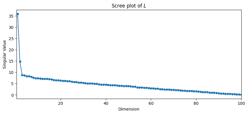
from scipy.linalg import svdvals

# use scipy to obtain the singular values
s = svdvals(A)

from pandas import DataFrame
import seaborn as sns
import matplotlib.pyplot as plt


def plot_scree(svs, title="", ax=None):
    """
    A utility to plot the scree plot for a list of singular values
    svs.
    """
    if ax is None:
        fig, ax = plt.subplots(1,1, figsize=(10, 4))
    sv_dat = DataFrame({"Singular Value": svs, "Dimension": range(1, len(svs) + 1)})
    sns.scatterplot(data=sv_dat, x="Dimension", y="Singular Value", ax=ax)
    sns.lineplot(data=sv_dat, x="Dimension", y="Singular Value", ax=ax)
    ax.set_xlim([0.5, len(s)])
    ax.set_title(title)

plot_scree(s, title="Scree plot of $L$")

from graspologic.embed import AdjacencySpectralEmbed as ase

# use automatic elbow selection
Xhat_auto = ase(svd_seed=0).fit_transform(A)

from graspologic.embed import AdjacencySpectralEmbed as ase
from scipy.spatial import distance_matrix

nk = 50  # the number of nodes in each community
B_indef = np.array([[.1, .5], [.5, .2]])
np.random.seed(0)
A_dis, z = sbm([nk, nk], B_indef, return_labels=True)
Xhat = ase(n_components=2, svd_seed=0).fit_transform(A_dis)
D = distance_matrix(Xhat, Xhat)