5.7 Estimating latent dimensionality and non positive semidefiniteness

mode = "svg"

import matplotlib

font = {'family' : 'Dejavu Sans',
        'weight' : 'normal',
        'size'   : 20}

matplotlib.rc('font', **font)

import matplotlib
from matplotlib import pyplot as plt

from graspologic.simulations import sbm
import numpy as np

# block matrix
n = 100
B = np.array([[0.6, 0.2], [0.2, 0.4]])
# network sample
np.random.seed(0)
A, z = sbm([n // 2, n // 2], B, return_labels=True)

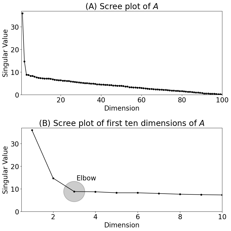
from scipy.linalg import svdvals

# use scipy to obtain the singular values
s = svdvals(A)

from pandas import DataFrame
import seaborn as sns
import matplotlib.pyplot as plt


def plot_scree(svs, title="", ax=None):
    """
    A utility to plot the scree plot for a list of singular values
    svs.
    """
    if ax is None:
        fig, ax = plt.subplots(1,1, figsize=(10, 4))
    sv_dat = DataFrame({"Singular Value": svs, "Dimension": range(1, len(svs) + 1)})
    sns.scatterplot(data=sv_dat, x="Dimension", y="Singular Value", ax=ax, color="black")
    sns.lineplot(data=sv_dat, x="Dimension", y="Singular Value", ax=ax, color="black")
    ax.set_xlim([0.5, len(svs)])
    ax.set_ylim([0, svs.max() + 1])
    ax.set_title(title)

from matplotlib.patches import Ellipse
import os

fig, axs = plt.subplots(2, 1, figsize=(10, 10))

plot_scree(s, ax=axs[0], title="(A) Scree plot of $A$")
plot_scree(s[0:10], ax=axs[1], title="(B) Scree plot of first ten dimensions of $A$")

x0, y0 = axs[1].transAxes.transform((0, 0)) # lower left in pixels
x1, y1 = axs[1].transAxes.transform((1, 1)) # upper right in pixes

r = 5
# Create a circle annotation
circle = Ellipse((3, s[2]), 1, 9, color='black', fill="gray", alpha=0.2, linewidth=2)
axs[1].add_patch(circle)
axs[1].annotate("Elbow", xy=(3.1, s[2] + 5))

fig.tight_layout()

os.makedirs("Figures", exist_ok=True)
fname = "scree"
if mode != "png":
    os.makedirs(f"Figures/{mode:s}", exist_ok=True)
    fig.savefig(f"Figures/{mode:s}/{fname:s}.{mode:s}")

os.makedirs("Figures/png", exist_ok=True)
fig.savefig(f"Figures/png/{fname:s}.png")

from graspologic.embed import AdjacencySpectralEmbed as ase

# use automatic elbow selection
Xhat_auto = ase(svd_seed=0).fit_transform(A)

from graspologic.embed import AdjacencySpectralEmbed as ase
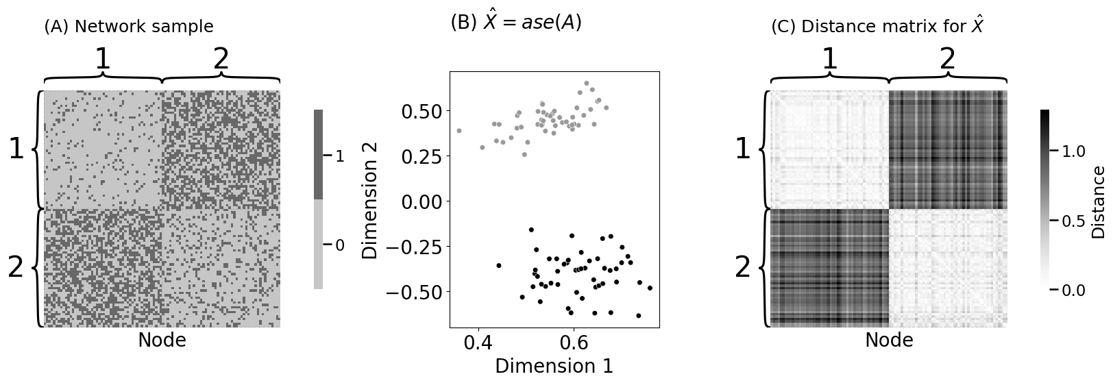
from scipy.spatial import distance_matrix

nk = 50  # the number of nodes in each community
B_indef = np.array([[.1, .5], [.5, .2]])
np.random.seed(0)
A_dis, z = sbm([nk, nk], B_indef, return_labels=True)
Xhat = ase(n_components=2, svd_seed=0).fit_transform(A_dis)
D = distance_matrix(Xhat, Xhat)

from graphbook_code import heatmap, plot_latents

fig, axs = plt.subplots(1, 3, figsize=(17, 6), gridspec_kw={"width_ratios": [1, .6, 1]})

heatmap(A_dis.astype(int), ax=axs[0], inner_hier_labels=z+1, title="(A) Network sample", xtitle="Node")
plot_latents(Xhat, labels=z + 1, palette={1: "#999999", 2: "#000000"}, title="(B) $\\hat X = ase(A)$", s=30, ax=axs[1])
axs[1].get_legend().remove()
axs[1].set_xlabel("Dimension 1")
axs[1].set_ylabel("Dimension 2")
axs[1].set_title("(B) $\\hat X = ase(A)$", pad=45, loc="left", fontsize=20)
heatmap(D, ax=axs[2], inner_hier_labels=z+1, title="(C) Distance matrix for $\\hat X$", xtitle="Node", legend_title="Distance")

fig.tight_layout()

fname = "diss"
if mode != "png":
    fig.savefig(f"Figures/{mode:s}/{fname:s}.{mode:s}")

fig.savefig(f"Figures/png/{fname:s}.png")