Code Reproducibility

import numpy as np
from graphbook_code import dcsbm

nk = 100  # 100 nodes per community
K = 3  # the number of communities
n = nk * K  # total number of nodes

zs = np.repeat(np.arange(K)+1, repeats=nk)
# block matrix and degree-correction factor
B = np.array([[0.7, 0.2, 0.1], [0.2, 0.5, 0.1], [0.1, 0.1, 0.4]])
theta = np.tile(np.linspace(start=0, stop=1, num=nk), reps=K)
# generate network sample
np.random.seed(0)
A = dcsbm(zs, theta, B)

# permute the nodes randomly
vtx_perm = np.random.choice(n, size=n, replace=False)
Aperm = A[vtx_perm, :][:,vtx_perm]
zperm = zs[vtx_perm]

import scipy as sp
from graspologic.embed import AdjacencySpectralEmbed as ase

Xhat = ase(n_components=3, svd_seed=0).fit_transform(Aperm)
D = sp.spatial.distance_matrix(Xhat, Xhat)

/opt/hostedtoolcache/Python/3.12.5/x64/lib/python3.12/site-packages/graspologic/embed/base.py:199: UserWarning: Input graph is not fully connected. Results may notbe optimal. You can compute the largest connected component byusing ``graspologic.utils.largest_connected_component``.
  warnings.warn(msg, UserWarning)

from sklearn.cluster import KMeans

labels_kmeans = KMeans(n_clusters = 3, random_state=0).fit_predict(Xhat)

from sklearn.metrics import confusion_matrix

# compute the confusion matrix between the true labels z
# and the predicted labels labels_kmeans
cf_matrix = confusion_matrix(zperm, labels_kmeans)

from sklearn.metrics import adjusted_rand_score

ari_kmeans = adjusted_rand_score(zperm, labels_kmeans)
print(ari_kmeans)
# 0.490

0.4901452495709552

from graspologic.utils import remap_labels

labels_kmeans_remap = remap_labels(zperm, labels_kmeans)

# compute which assigned labels from labels_kmeans_remap differ from the true labels z
error = zperm - labels_kmeans_remap
# if the difference between the community labels is non-zero, an error has occurred
error = error != 0
error_rate = np.mean(error)  # error rate is the frequency of making an error

Xhat = ase(svd_seed=0).fit_transform(Aperm)
print("Estimated number of dimensions: {:d}".format(Xhat.shape[1]))
# Estimated number of dimensions: 3

Estimated number of dimensions: 3

/opt/hostedtoolcache/Python/3.12.5/x64/lib/python3.12/site-packages/graspologic/embed/base.py:199: UserWarning: Input graph is not fully connected. Results may notbe optimal. You can compute the largest connected component byusing ``graspologic.utils.largest_connected_component``.
  warnings.warn(msg, UserWarning)

from graspologic.cluster import KMeansCluster

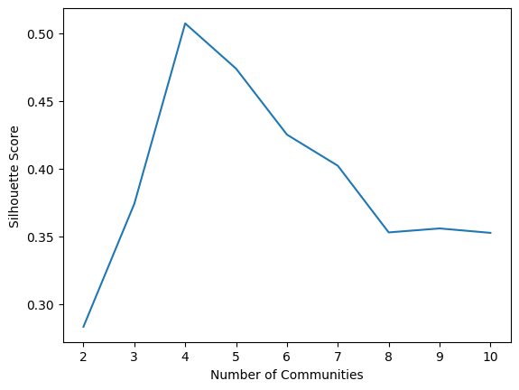
km_clust = KMeansCluster(max_clusters = 10, random_state=0)
labels_kmclust = km_clust.fit_predict(Xhat)

import seaborn as sns
from pandas import DataFrame as df

nclusters = range(2, 11)  # graspologic nclusters goes from 2 to max_clusters
silhouette = km_clust.silhouette_ # obtain the respective silhouettes

# place into pandas dataframe
ss_df = df({"Number of Communities": nclusters, "Silhouette Score": silhouette})
sns.lineplot(data=ss_df, x="Number of Communities", y="Silhouette Score")

<Axes: xlabel='Number of Communities', ylabel='Silhouette Score'>

import numpy as np
from graspologic.simulations import sample_edges
from graphbook_code import generate_sbm_pmtx
    
def academic_pmtx(K, nk=10, return_zs=False):
    """
    Produce probability matrix for academic example.
    """
    n = K*nk
    # get the community assignments
    zs = np.repeat(np.arange(K)+1, repeats=nk)
    # randomly generate proteges and lab leaders
    unif_choices = np.random.uniform(size=n)
    thetas = np.zeros(n)
    # 90% are proteges
    thetas[unif_choices > .1] = np.random.beta(1, 5, size=(unif_choices > .1).sum())
    # 10% are lab leaders
    thetas[unif_choices <= .1] = np.random.beta(2, 1, size=(unif_choices <= .1).sum())
    # define block matrix
    B = np.full(shape=(K,K), fill_value=0.01)
    np.fill_diagonal(B, 1)
    # generate probability matrix for SBM
    Pp = generate_sbm_pmtx(zs, B)
    Theta = np.diag(thetas)
    # adjust probability matrix for SBM by degree-corrections
    P = Theta @ Pp @ Theta.transpose()
    if return_zs:
        return P, zs
    return P

def academic_example(K, nk=10, return_zs=False):
    P = academic_pmtx(K, nk=nk, return_zs=return_zs)
    if return_zs:
        return (sample_edges(P[0]), P[1])
    else:
        return sample_edges(P)

import pandas as pd
from tqdm import tqdm  # optional

results = []
nrep = 50
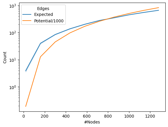
for K in tqdm(np.linspace(start=2, stop=128, num=10, dtype=int)):
    for j in range(nrep):
        P = academic_pmtx(K)
        n = P.shape[0]
        results.append({"Count": np.triu(P, k=1).sum(), "Edges": "Expected", 
                        "#Nodes": n, "Index": j})
        results.append({"Count": n*(n - 1)/2000, "Edges": "Potential/1000",
                        "#Nodes": n, "Index": j})

df = pd.DataFrame(results)
df_mean=df.groupby(["Edges", "#Nodes"])[["Count"]].mean()

  0%|          | 0/10 [00:00<?, ?it/s]

 30%|███       | 3/10 [00:00<00:00, 20.60it/s]

 60%|██████    | 6/10 [00:02<00:01,  2.48it/s]

 70%|███████   | 7/10 [00:03<00:02,  1.41it/s]

 80%|████████  | 8/10 [00:06<00:02,  1.18s/it]

 90%|█████████ | 9/10 [00:10<00:01,  1.88s/it]

100%|██████████| 10/10 [00:15<00:00,  2.78s/it]

100%|██████████| 10/10 [00:15<00:00,  1.58s/it]

ax = sns.lineplot(data=df, x="#Nodes", y="Count", hue="Edges")
ax.set(yscale="log")

[None]

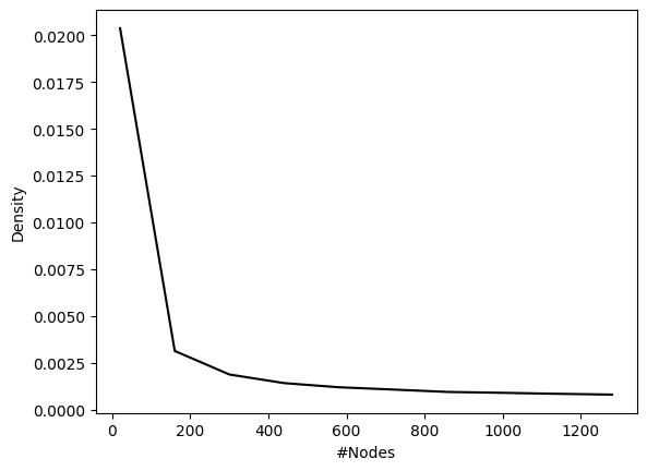
df_wide = pd.pivot(df_mean.reset_index(), index="#Nodes", columns="Edges", values="Count")
# remember normalizing constant of 100 for potential edges
df_wide["Density"] = df_wide["Expected"]/(1000*df_wide["Potential/1000"])
df_wide = df_wide.reset_index()
# plot it
sns.lineplot(data=df_wide, x="#Nodes", y="Density", color="black")

<Axes: xlabel='#Nodes', ylabel='Density'>

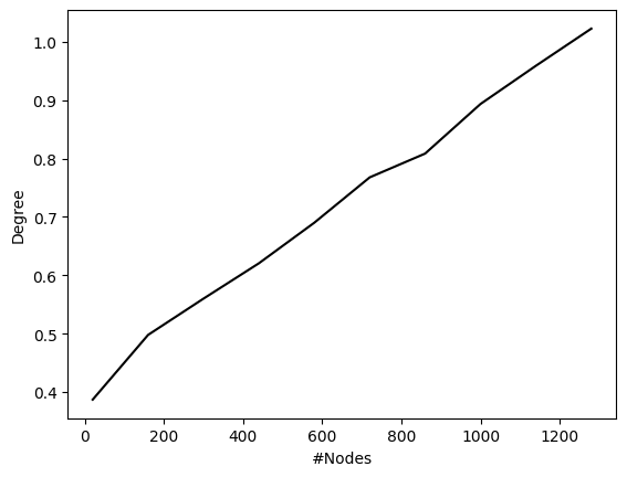
df_wide["Degree"] = df_wide["Density"]*(df_wide["#Nodes"] - 1)
sns.lineplot(data=df_wide, x="#Nodes", y="Degree", color="black")

<Axes: xlabel='#Nodes', ylabel='Degree'>

np.random.seed(0)
K = 10; nk = 100
P, zs = academic_example(K, nk=nk, return_zs=True)
A = sample_edges(P)

print(f"# Non-zero entries: {A.sum().astype(int)}")  
# Non-zero entries: 5308

print(f"# Number of entries: {A.size}")  
# Number of entries: 1000000

# Non-zero entries: 5308
# Number of entries: 1000000

print(f"Size in KB: {A.nbytes/1000:.3f} KB")
# Size in KB: 8000.000 KB

B = A.astype(np.uint8)
print(f"Size in KB: {B.nbytes/1000:.3f} KB")
# Size in KB: 1000.000 KB

Size in KB: 8000.000 KB
Size in KB: 1000.000 KB

import scipy.sparse as sparse

Btriu = sparse.triu(B)
print(f"Size in KB: {Btriu.data.size/1000:.3f}")
# Size in KB: 2.654 KB

Size in KB: 2.654

Btriu
# <1000x1000 sparse matrix of type '<class 'numpy.uint8'>'
#     with 2654 stored elements in COOrdinate format>

<1000x1000 sparse matrix of type '<class 'numpy.uint8'>'
	with 2654 stored elements in COOrdinate format>

from graspologic.utils import symmetrize

# cast the sparse matrix back to a dense matrix,
# and then triu symmetrize with graspologic
A_new = symmetrize(Btriu.todense(), method="triu")
np.array_equal(A_new, A)  # True

True

import time
import scipy as sp

# a naive full svd on the dense matrix
timestart = time.time()
U, S, Vh = sp.linalg.svd(A)
Xhat = U[:, 0:10] @ np.diag(np.sqrt(S[0:10]))
timeend = time.time()
print(f"Naive approach: {timeend - timestart:3f} seconds")
# we get about 0.55 seconds

# a sparse svd on the sparse matrix
Acoo = sparse.coo_array(A)
timestart = time.time()
U, S, Vh = sp.sparse.linalg.svds(Acoo, k=10)
Xhat = U @ np.diag(np.sqrt(S))
timeend = time.time()
print(f"Sparse approach: {timeend-timestart:3f} seconds")
# we get about .01 seconds

Naive approach: 0.240999 seconds
Sparse approach: 0.017672 seconds

degrees = A.sum(axis=0)

from graspologic.utils import to_laplacian
from graspologic.plot import pairplot

# use sparse svd, so that we don't need to compute
# 1000 singular vectors and can just calculate the top 10
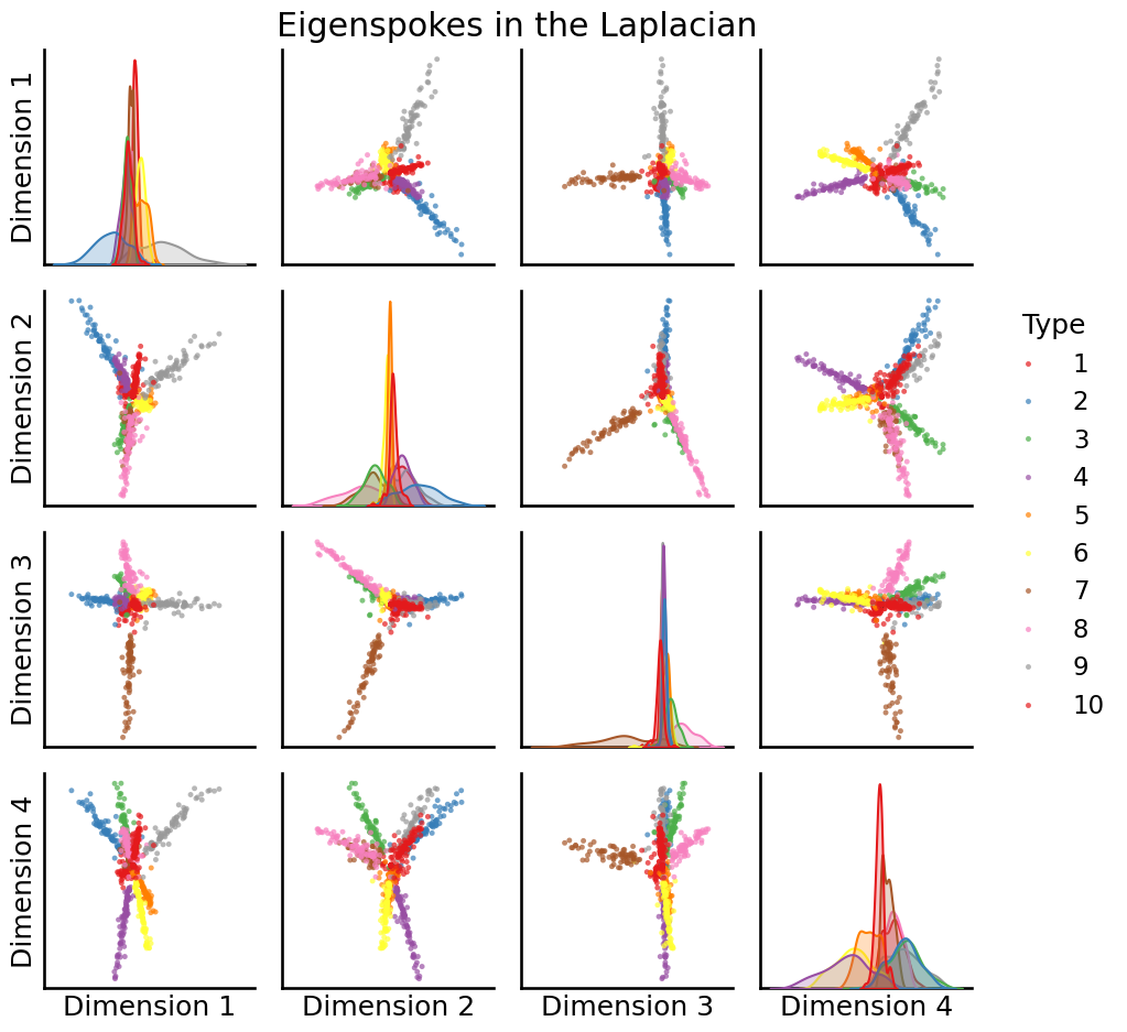
U, S, Vh = sp.sparse.linalg.svds(to_laplacian(A), k=10, random_state=0)
# plot the first 4
pairplot(U[:,0:4], labels=zs, title="Eigenspokes in the Laplacian")

<seaborn.axisgrid.PairGrid at 0x7f5a50caaf30>

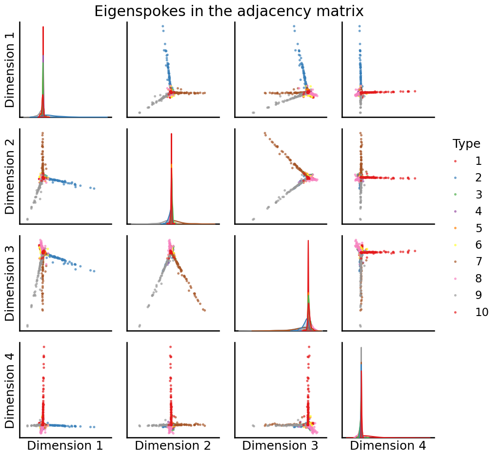
U, S, Vh = sp.sparse.linalg.svds(A, k=10, random_state=0)
# plot the first 4
fig = pairplot(U[:,0:4], labels=zs, title="Eigenspokes in the adjacency matrix")

print("# Expected edges: {:.2f}".format(np.triu(P).sum()))
# Expected edges: 2654.00
print("# True edges: {:d}".format(np.triu(A).sum().astype(int)))
# True edges: 2654
print("# Potential edges: {:d}".format(int(K*nk*(K*nk - 1)/2)))
# Potential edges: 499500

# Expected edges: 2654.00
# True edges: 2654
# Potential edges: 499500

import numpy as np
from graphbook_code import siem

n = 100
Z = np.ones((n, n))

# Fill the upper and lower 50th diagonals with 2
# and the main diagonal with 0
np.fill_diagonal(Z[:, 50:], 2)
np.fill_diagonal(Z[50:, :], 2)
np.fill_diagonal(Z, 0)

p = [0.4, 0.6]
np.random.seed(0)
A = siem(n, p, Z)

est_pvec = {k: A[Z == k].mean() for k in [1, 2]}
print(est_pvec)
# {1: 0.3955102040816327, 2: 0.6}

{1: 0.3955102040816327, 2: 0.6}

from scipy.stats import fisher_exact
import numpy as np

# assemble the contingency table indicated
table = np.array([[3, 7], [7, 3]])
_, pvalue = fisher_exact(table)
print(f"p-value: {pvalue:.3f}")
# p-value: 0.179

p-value: 0.179

# compute an upper-triangular mask to only look at the
# upper triangle since the network is simple (undirected and loopless)
upper_tri_mask = np.triu(np.ones(A.shape), k=1).astype(bool)
column_clust1 = [
    A[(Z == 1) & upper_tri_mask].sum(),
    (A[(Z == 1) & upper_tri_mask] == 0).sum(),
]
column_clust2 = [
    A[(Z == 2) & upper_tri_mask].sum(),
    (A[(Z == 2) & upper_tri_mask] == 0).sum(),
]
cont_tabl = np.vstack((column_clust1, column_clust2))

_, pvalue = fisher_exact(cont_tabl)
print(f"p-value: {pvalue:.5f}")
# p-value: 0.00523

p-value: 0.00523

import numpy as np
from graspologic.simulations import sbm

nk = 50  # 50 nodes per community
K = 2  # the number of communities
n = nk * K  # total number of nodes

zs = np.repeat(np.arange(1, K+1), repeats=nk)
# block matrix
B = np.array([[0.6, 0.3],[0.3, 0.5]])
# generate network sample
np.random.seed(0)
A = sbm([nk, nk], B)

from graspologic.models import SBMEstimator

# instantiate the class object and fit
model = SBMEstimator(directed=False, loops=False)
model.fit(A, y=zs)
# obtain the estimate of the block matrix
Bhat = model.block_p_

# upper left has a value of 1, lower right has a value of 2,
# and upper right, bottom left have a value of 3
Z = np.array(zs).reshape(n, 1) @ np.array(zs).reshape(1, n)
# make lower right have a value of 3
Z[Z == 4] = 3

import statsmodels.api as sm
import pandas as pd
import statsmodels.formula.api as smf
from scipy import stats as spstat

# upper triangle since the network is simple (undirected and loopless)
upper_tri_non_diag = np.triu(np.ones(A.shape), k=1).astype(bool)

df_H1 = pd.DataFrame({"Value" : A[upper_tri_non_diag],
            "Group": (Z[upper_tri_non_diag] != 2).astype(int)})

# fit the logistic regression model, regressing the outcome (edge or no edge)
# onto the edge group (on-diagonal or off-diagonal), the grouping
# corresponding to H1
model_H1 = smf.logit("Value ~ C(Group)", df_H1).fit()

# compare the likelihood ratio statistic to the chi2 distribution
# with 1 dof to see the fraction that is less than l1
dof = 1
print(f"p-value: {spstat.chi2.sf(model_H1.llr, dof):.3f}")
# p-value: 0.00000

Optimization terminated successfully.
         Current function value: 0.651736
         Iterations 5
p-value: 0.000

df_H2 = pd.DataFrame({"Value": A[upper_tri_non_diag],
                      "Group": Z[upper_tri_non_diag].astype(int)})
model_H2 = smf.logit("Value ~ C(Group)", df_H2).fit()
lr_stat_H2vsH1 = model_H2.llr - model_H1.llr
print(f"p-value: {spstat.chi2.sf(lr_stat_H2vsH1, 1):.7f}")
# 0.00008

Optimization terminated successfully.
         Current function value: 0.650168
         Iterations 5
p-value: 0.0000813

import numpy as np
from graspologic.simulations import sbm

# first 100 nodes are traffickers, second 900 are non-traffickers
ns = [100, 900]
B = np.array([[0.3, 0.1], [0.1, 0.2]])
np.random.seed(0)
A = sbm(ns, B)

# the number of seed nodes
nseeds = 20
# The first ns[0] nodes are the human traffickers, so choose 20 seeds
# at random
seed_ids = np.random.choice(ns[0], size=20)

from graspologic.embed import AdjacencySpectralEmbed as ase

Xhat = ase(n_components=2, svd_seed=0).fit_transform(A)

from sklearn.cluster import KMeans

# community detection with kmeans
km_clust = KMeans(n_clusters=2, random_state=0)
km_clust.fit(Xhat)
labels_kmeans = km_clust.fit_predict(Xhat)

from graphbook_code import ohe_comm_vec

# estimated community assignment matrix
Chat = ohe_comm_vec(labels_kmeans)

# get the community (class) with the most seeds
comm_of_seeds = np.argmax(Chat[seed_ids,:].sum(axis=0))

# get centroid of the community that seeds tend to be
# assigned to
centroid_seeds = km_clust.cluster_centers_[comm_of_seeds]

from scipy.spatial.distance import cdist
from scipy.stats import rankdata

# compute the distance to the centroid for all estimated latent positions
dists_to_centroid = cdist(Xhat, centroid_seeds.reshape(1, -1)).reshape(-1)
# compute the node numbers for all the nonseed nodes
nonseed_bool = np.ones((np.sum(ns)))
nonseed_bool[seed_ids] = 0
nonseed_ids = np.array(np.where(nonseed_bool)).reshape(-1)

# isolate the distances to the centroid for the nonseed nodes
nonseed_dists = dists_to_centroid[nonseed_ids]

# produce the nomination list
nom_list_nonseeds = np.argsort(nonseed_dists).reshape(-1)
# obtain a nomination list in terms of the original node ids
nom_list = nonseed_ids[nom_list_nonseeds]

import numpy as np
from graspologic.simulations import sbm

# the in-sample nodes
n = 100
nk = 50
# the out-of-sample nodes
np1 = 1; np2 = 2
B = np.array([[0.6, 0.2], [0.2, 0.4]])
# sample network
np.random.seed(0)
A, zs = sbm([nk + np1, nk + np2], B, return_labels=True)

from graspologic.utils import remove_vertices

# the indices of the out-of-sample nodes
oos_idx = [nk, nk + np1 + nk, nk + np1 + nk + 1]
# get adjacency matrix and the adjacency vectors A prime
Ain, Aoos = remove_vertices(A, indices=oos_idx, return_removed=True)

from graspologic.embed import AdjacencySpectralEmbed as ase

oos_embedder = ase()
# estimate latent positions for the in-sample nodes
# using the subnetwork induced by the in-sample nodes
Xhat_in = oos_embedder.fit_transform(Ain)

Xhat_oos = oos_embedder.transform(Aoos)