B.1 The basics of maximum likelihood estimation

mode = "svg"

import matplotlib

font = {'family' : 'Dejavu Sans',
        'weight' : 'normal',
        'size'   : 20}

matplotlib.rc('font', **font)

import matplotlib
from matplotlib import pyplot as plt

import numpy as np

p = np.linspace(.02, .98, num=49)
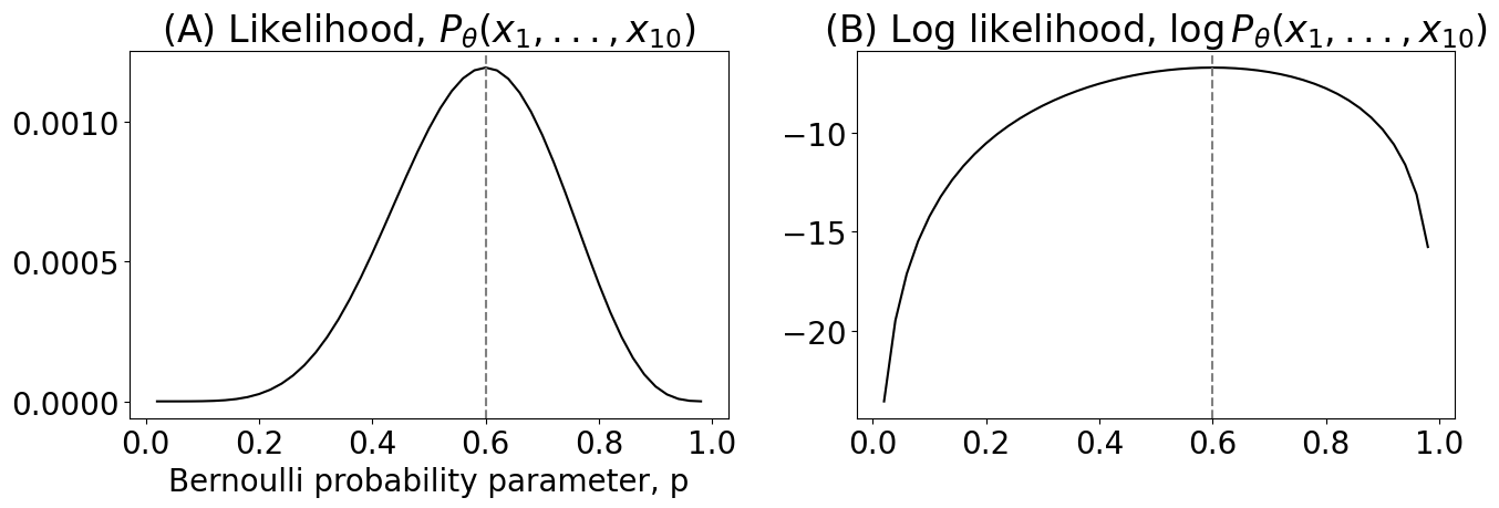
nflips = 10; nheads = 6
likelihood = p**(nheads)*(1 - p)**(nflips - nheads)

loglikelihood = nheads*np.log(p) + (nflips - nheads)*np.log(1 - p)

import seaborn as sns
import matplotlib.pyplot as plt
import os

fig, axs = plt.subplots(1, 2, figsize=(14, 5))
sns.lineplot(x=p, y=likelihood, ax=axs[0], color="black")
axs[0].axvline(.6, color="gray", linestyle="--")
axs[0].set(xlabel="Bernoulli probability parameter, p", title="(A) Likelihood, $P_{\\theta}(x_1, ..., x_{10})$");

sns.lineplot(x=p, y=loglikelihood, ax=axs[1], color="black")
axs[1].axvline(.6, color="gray", linestyle="--")
axs[1].set(xlabel="", title="(B) Log likelihood, $\\log P_{\\theta}(x_1, ..., x_{10})$");

fig.tight_layout()

os.makedirs("Figures", exist_ok=True)
fname = "mle_coin"
if mode != "png":
    os.makedirs(f"Figures/{mode:s}", exist_ok=True)
    fig.savefig(f"Figures/{mode:s}/{fname:s}.{mode:s}")

os.makedirs("Figures/png", exist_ok=True)
fig.savefig(f"Figures/png/{fname:s}.png")

import scipy as sp

# simulation of 1000 values from the N(0,1) distn
n = 1000
xs = np.random.normal(loc=0, scale=1, size=n)
ys = np.random.normal(loc=0, scale=1, size=n)
# compute the square
xssq = xs**2
yssq = ys**2
sum_xsq_ysq = xssq + yssq

# compute the centers for bin histograms from 0 to maxval in
# 30 even bins
nbins = 30
bincenters = np.linspace(start=0, stop=np.max(sum_xsq_ysq), num=nbins)

# compute the pdf of the chi-squared distribution for X^2 + Y^2, which when
# X, Y are N(0, 1), is Chi2(2), the chi-squared distn with 2 degrees of freedom
dof = 2
true_pdf = sp.stats.chi2.pdf(bincenters, dof)

from graspologic.simulations import er_np
from graspologic.models import EREstimator

n = 10  # number of nodes
nsims = 200  # number of networks to simulate
p = 0.4

As = [er_np(n, p, directed=False, loops=False) for i in range(0, nsims)]  # realizations
fit_models = [EREstimator(directed=False, loops=False).fit(A) for A in As]  # fit ER models
hatps = [model.p_ for model in fit_models]  # the probability parameters

from pandas import DataFrame

fig, axs = plt.subplots(1,2, figsize=(18, 5))

df = DataFrame({"x": bincenters, "y": true_pdf})
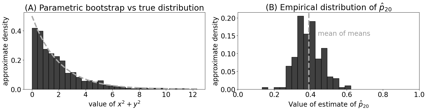
sns.histplot(sum_xsq_ysq, bins=30, ax=axs[0], stat = "density", color="black")
sns.lineplot(x="x", y="y", data=df, ax=axs[0], color="#AAAAAA", linestyle="--", linewidth=4)
axs[0].set_xlabel("value of $x^2 + y^2$")
axs[0].set_ylabel("approximate density")
axs[0].set_title("(A) Parametric bootstrap vs true distribution");

sns.histplot(hatps, bins=15, ax=axs[1], stat="probability", color="black")
axs[1].set_xlim(0, 1)
axs[1].set_ylabel("approximate density")
axs[1].axvline(np.mean(hatps), color="#AAAAAA", linestyle="--", linewidth=4)
axs[1].text(x=np.mean(hatps) + .05, y=.15, s="mean of means", color="#999999");
axs[1].set_title("(B) Empirical distribution of ${\\hat p}_{20}$")
axs[1].set_xlabel("Value of estimate of $\\hat p_{20}$")

fig.tight_layout()

fname = "mle_param_bootstrap"
if mode != "png":
    fig.savefig(f"Figures/{mode:s}/{fname:s}.{mode:s}")

fig.savefig(f"Figures/png/{fname:s}.png")

from pandas import DataFrame
import graspologic as gp

ns = [8, 16, 32, 64, 128]
nsims = 200
p = 0.4

results = []
for n in ns:
    for i in range(0, nsims):
        A = gp.simulations.er_np(n, p, directed=False, loops=False)
        phatni = gp.models.EREstimator(directed=False, loops=False).fit(A).p_
        results.append({"n": n, "i": i, "phat": phatni})

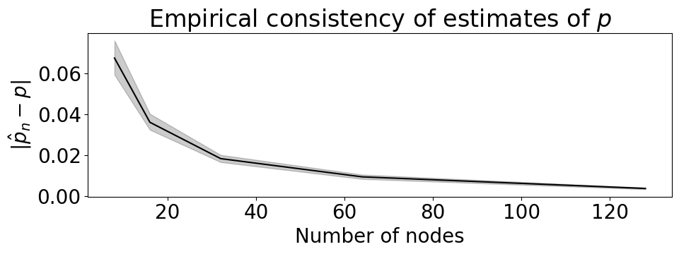
res_df = DataFrame(results)
res_df["diff"] = np.abs(res_df["phat"] - p)

fig, ax = plt.subplots(1,1, figsize=(10, 4))

sns.lineplot(data=res_df, x="n", y="diff", ax=ax, color="black")
ax.set_title("Empirical consistency of estimates of $p$")
ax.set_xlabel("Number of nodes")
ax.set_ylabel("$|\\hat p_n - p|$");

fig.tight_layout()
fname = "mle_asy_cons"
if mode != "png":
    fig.savefig(f"Figures/{mode:s}/{fname:s}.{mode:s}")

fig.savefig(f"Figures/png/{fname:s}.png")