8.2 Testing for significant edges in incoherent signal subnetworks#
mode = "svg"

import matplotlib

font = {'family' : 'Dejavu Sans',
        'weight' : 'normal',
        'size'   : 20}

matplotlib.rc('font', **font)

import matplotlib
from matplotlib import pyplot as plt
import numpy as np

pi_astronaut = 0.45
pi_earthling = 0.55
M = 200

# roll a 2-sided die 200 times, with probability 0.45 of landing on side 2 (astronaut)
# and probability 0.55 of landing on side 1 (earthling)
classnames = ["Earthling", "Earthling"]
np.random.seed(0)
ys = np.random.choice([1, 2], p=[pi_earthling, pi_astronaut], size=M)
print(f"Number of individuals who are earthlings: {(ys == 1).sum():d}")
print(f"Number of individuals who are astronauts: {(ys == 2).sum():d}")
Number of individuals who are earthlings: 102
Number of individuals who are astronauts: 98
n = 5
P_earthling = np.full(shape=(n, n), fill_value=0.3)
nodenames = [
"SI", "L", "H/E",
"T/M", "BS"
]
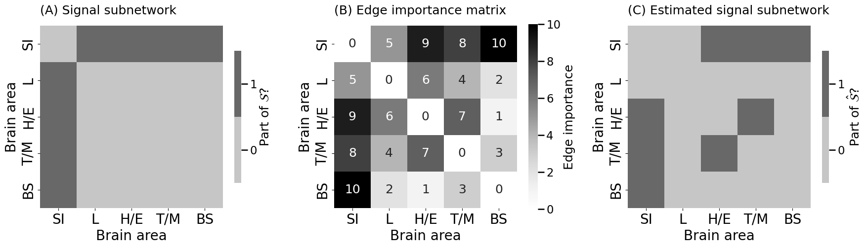
signal_subnetwork = np.full(shape=(n, n), fill_value=False)
signal_subnetwork[1:n, 0] = True
signal_subnetwork[0, 1:n] = True
P_astronaut = np.copy(P_earthling)
# probabilities for signal edges are higher in astronauts than earthlings
P_astronaut[signal_subnetwork] = np.tile(np.linspace(0.4, 0.9, num=4), reps=2)
from graspologic.simulations import sample_edges

# the probability matrices for each class
Ps = [P_earthling, P_astronaut]

# sample networks with the indicated probability matrix
np.random.seed(0)
As = np.stack([sample_edges(P=Ps[y-1]) for y in ys], axis=2)
def generate_table(As, ys, i, j):
    """
    A function to generate a contingency table for a given edge.
    """
    # count the number of earthlings with edge i,j
    a = As[i,j,ys == 1].sum()
    # count the number of astronauts with edge i,j
    b = As[i,j,ys == 2].sum()

    c = len(As[i,j,ys == 1]) - a
    d = len(As[i,j,ys == 2]) - b

    edge_tab = np.array([[a, b], [c, d]])
    return edge_tab

# edge (0, 4) corresponds to SI to BS
edge_tab = generate_table(As, ys, 0, 4)
print(edge_tab)
[[29. 86.]
 [73. 12.]]
from scipy.stats import fisher_exact

_, pval = fisher_exact(edge_tab)
print(f"p-value: {pval:.4f}")
# p-value: 0.0000
p-value: 0.0000
_, pval = fisher_exact(generate_table(As, ys, 2, 1))
print(f"p-value: {pval:.4f}")
# p-value: 0.7600
p-value: 0.7600
from graspologic.utils import symmetrize
from scipy.stats import rankdata

fisher_mtx = np.empty((n, n))
fisher_mtx[:] = np.nan

for i in range(0, n):
    for j in range(i+1, n):
        fisher_mtx[i, j] = fisher_exact(generate_table(As, ys, i, j))[1]
fisher_mtx = symmetrize(fisher_mtx, method="triu")
# use rankdata on -fisher_mtx, to rank from largest p-value to smallest p-value
edge_imp = rankdata(-fisher_mtx, method="dense", nan_policy="omit").reshape(fisher_mtx.shape)
np.fill_diagonal(edge_imp, 0)
from graspologic.subgraph import SignalSubgraph

K = 8  # the number of edges in the subgraph
ssn_mod = SignalSubgraph()
# graspologic signal subgraph module assumes labels are 0, ..., K-1
# so use ys - 1 to rescale from (1, 2) to (0, 1)
ssn_mod.fit_transform(As, labels=ys - 1, constraints=K);

sn_est = np.zeros((n,n))  # initialize empty matrix
sn_est[ssn_mod.sigsub_] = 1
import os
from graphbook_code import heatmap

fig, axs = plt.subplots(1, 3, figsize=(18, 6))

heatmap(signal_subnetwork.astype(int), ax = axs[0], title="(A) Signal subnetwork",
        xtitle="Brain area", ytitle="Brain area", xticklabels=nodenames, yticklabels=nodenames, shrink=0.5,
        legend_title="Part of $\\mathcal{S}$?")
heatmap(edge_imp, ax = axs[1], title="(B) Edge importance matrix",
        xtitle="Brain area", ytitle="Brain area", xticklabels=nodenames, yticklabels=nodenames,
        legend_title="Edge importance", annot=True)
heatmap(sn_est.astype(int), ax = axs[2], title="(C) Estimated signal subnetwork",
        xtitle="Brain area", ytitle="Brain area", shrink=0.5, xticklabels=nodenames, yticklabels=nodenames,
        legend_title="Part of $\\hat{\\mathcal{S}}$?")
fig.tight_layout()

fname = "ssn_inco_edgeimp"
if mode != "png":
    os.makedirs(f"Figures/{mode:s}", exist_ok=True)
    fig.savefig(f"Figures/{mode:s}/{fname:s}.{mode:s}")

os.makedirs("Figures/png", exist_ok=True)
fig.savefig(f"Figures/png/{fname:s}.png")
D = As[ssn_mod.sigsub_[0], ssn_mod.sigsub_[1],:].T
from sklearn.naive_bayes import BernoulliNB

classifier = BernoulliNB()
# fit the classifier using the vector of classes for each sample
classifier.fit(D, ys)
BernoulliNB()In a Jupyter environment, please rerun this cell to show the HTML representation or trust the notebook.
On GitHub, the HTML representation is unable to render, please try loading this page with nbviewer.org.
BernoulliNB()
# number of holdout samples
Mp = 200
# new random seed so heldout samples differ
np.random.seed(123)
y_heldout = np.random.choice([1, 2], p=[pi_earthling, pi_astronaut], size=Mp)
# sample networks with the appropriate probability matrix
A_heldout = np.stack([sample_edges(Ps[y-1]) for y in y_heldout], axis=2)

# compute testing data on the estimated signal subnetwork
D_heldout = A_heldout[ssn_mod.sigsub_[0], ssn_mod.sigsub_[1],:].T

yhat_heldout = classifier.predict(D_heldout)

# classifier accuracy is the fraction of predictions that are correct
heldout_acc = np.mean(yhat_heldout == y_heldout)
print(f"Classifier Testing Accuracy: {heldout_acc:.3f}")
Classifier Testing Accuracy: 0.810
def train_and_eval_ssn(Atrain, ytrain, Atest, ytest, K):
    """
    A function which trains and tests an incoherent signal subnetwork
    classifier with K signal edges.
    """
    ssn_mod = SignalSubgraph()
    ssn_mod.fit_transform(Atrain, labels=ytrain - 1, constraints=int(K));

    Dtrain = Atrain[ssn_mod.sigsub_[0], ssn_mod.sigsub_[1],:].T
    classifier = BernoulliNB()
    # fit the classifier using the vector of classes for each sample
    classifier.fit(Dtrain, ytrain)

    # compute testing data on the estimated signal subnetwork
    Dtest = Atest[ssn_mod.sigsub_[0], ssn_mod.sigsub_[1],:].T
    yhat_test = classifier.predict(Dtest)

    # classifier accuracy is the fraction of predictions that are correct
    return (np.mean(yhat_test == ytest), ssn_mod, classifier)
from sklearn.model_selection import KFold
import pandas as pd
from tqdm import tqdm

kf = KFold(n_splits=20, shuffle=True, random_state=0)
xv_res = []
for l, (train_index, test_index) in tqdm(enumerate(kf.split(range(0, M)))):
    A_train, A_test = As[:,:,train_index], As[:,:,test_index]
    y_train, y_test = ys[train_index], ys[test_index]
    nl = len(test_index)

    for k in np.arange(2, 20, step=2):
        acc_kl, _, _ = train_and_eval_ssn(A_train, y_train, A_test, y_test, k)
        xv_res.append({"Fold": l, "k": k, "nl": nl, "Accuracy": acc_kl})
xv_data = pd.DataFrame(xv_res)

def weighted_avg(group):
    acc = group['Accuracy']
    nl = group['nl']
    return (acc * nl).sum() / nl.sum()

xv_acc = xv_data.groupby(["k"]).apply(weighted_avg)
print(xv_acc)
0it [00:00, ?it/s]
1it [00:00, 5.90it/s]
2it [00:00, 4.94it/s]
3it [00:00, 4.92it/s]
4it [00:00, 5.14it/s]
5it [00:00, 4.97it/s]
6it [00:01, 4.81it/s]
7it [00:01, 4.82it/s]
8it [00:01, 5.26it/s]
9it [00:01, 5.21it/s]
10it [00:01, 5.26it/s]
11it [00:02, 5.35it/s]
12it [00:02, 5.40it/s]
13it [00:02, 5.55it/s]
14it [00:02, 5.61it/s]
15it [00:02, 5.33it/s]
16it [00:03, 5.39it/s]
17it [00:03, 5.35it/s]
18it [00:03, 5.25it/s]
19it [00:03, 5.19it/s]
20it [00:03, 5.41it/s]
20it [00:03, 5.26it/s]
k
2     0.795
4     0.795
6     0.830
8     0.830
10    0.820
12    0.825
14    0.825
16    0.820
18    0.820
dtype: float64
/tmp/ipykernel_2757/2121804480.py:22: DeprecationWarning: DataFrameGroupBy.apply operated on the grouping columns. This behavior is deprecated, and in a future version of pandas the grouping columns will be excluded from the operation. Either pass `include_groups=False` to exclude the groupings or explicitly select the grouping columns after groupby to silence this warning.
  xv_acc = xv_data.groupby(["k"]).apply(weighted_avg)