Code Reproducibility

import numpy as np
from graphbook_code import heatmap

def generate_unit_circle(radius):
    diameter = 2*radius + 1
    rx = ry = diameter/2
    x, y = np.indices((diameter, diameter))

    circle_dist = np.hypot(rx - x, ry - y)
    diff_from_radius = np.abs(circle_dist - radius)
    less_than_half = diff_from_radius < 0.5

    return less_than_half.astype(int)

def add_smile():
    canvas = np.zeros((51, 51))
    canvas[2:45, 2:45] = generate_unit_circle(21)
    mask = np.zeros((51, 51), dtype=bool)
    mask[np.triu_indices_from(mask)] = True
    upper_left = np.rot90(mask)
    canvas[upper_left] = 0
    return canvas
    
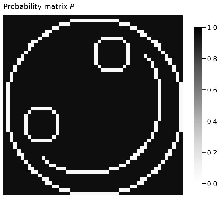
def smile_probability(upper_p, lower_p):
    smiley = add_smile()
    P = generate_unit_circle(25)
    P[5:16, 25:36] = generate_unit_circle(5)
    P[smiley != 0] = smiley[smiley != 0]
    
    mask = np.zeros((51, 51), dtype=bool)
    mask[np.triu_indices_from(mask)] = True
    P[~mask] = 0
    # symmetrize the probability matrix
    P = (P + P.T - np.diag(np.diag(P))).astype(float)
    P[P == 1] = lower_p
    P[P == 0] = upper_p
    return P

P = smile_probability(.95, 0.05)
heatmap(P, vmin=0, vmax=1, title="Probability matrix $P$")

<Axes: title={'left': 'Probability matrix $P$'}>

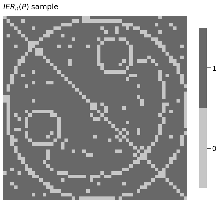
from graspologic.simulations import sample_edges

A = sample_edges(P, directed=False, loops=False)
heatmap(A.astype(int), title="$IER_n(P)$ sample")

<Axes: title={'left': '$IER_n(P)$ sample'}>

import numpy as np
from math import comb

node_count = np.arange(2, 51)
log_unique_network_count = np.array([comb(n, 2) for n in node_count])*np.log10(2)

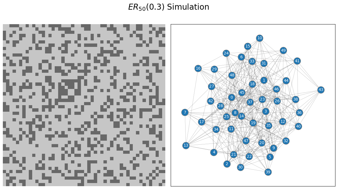
from graphbook_code import draw_multiplot
from graspologic.simulations import er_np

n = 50  # network with 50 nodes
p = 0.3  # probability of an edge existing is .3

# sample a single simple adjacency matrix from ER(50, .3)
A = er_np(n=n, p=p, directed=False, loops=False)

# and plot it
draw_multiplot(A.astype(int), title="$ER_{50}(0.3)$ Simulation")

array([<Axes: >, <Axes: >], dtype=object)

p = 0.7  # network has an edge probability of 0.7

# sample a single adjacency matrix from ER(50, 0.7)
A = er_np(n=n, p=p, directed=False, loops=False)

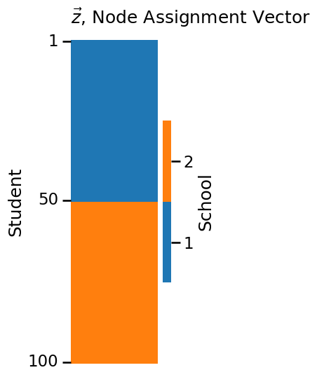
from graphbook_code import plot_vector
import numpy as np

n = 100  # number of students

# z is a column vector of 50 1s followed by 50 2s
# this vector gives the school each of the 100 students are from
z = np.repeat([1, 2], repeats=n//2)
plot_vector(z, title="$\\vec z$, Node Assignment Vector",
            legend_title="School", color="qualitative", 
            ticks=[0.5, 49.5, 99.5], ticklabels=[1, 50, 100],
            ticktitle="Student")

<Axes: title={'left': '$\\vec z$, Node Assignment Vector'}, ylabel='Student'>

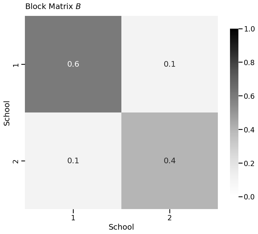
from graphbook_code import heatmap

K = 2  # community count
# construct the block matrix B as described above
B = np.array([[0.6, 0.1], 
              [0.1, 0.4]])

heatmap(B, xticklabels=[1, 2], yticklabels=[1,2], vmin=0, 
             vmax=1, annot=True, xtitle="School",
             ytitle="School", title="Block Matrix $B$")

<Axes: title={'left': 'Block Matrix $B$'}, xlabel='School', ylabel='School'>

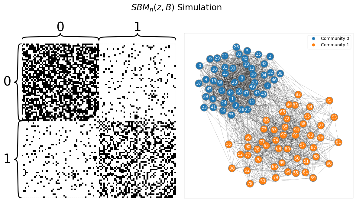
from graspologic.simulations import sbm
from graphbook_code import draw_multiplot

# sample a graph from SBM_{100}(tau, B)
A, labels = sbm(n=[n//2, n//2], p=B, directed=False, loops=False, return_labels=True)
draw_multiplot(A, labels=labels, title="$SBM_n(z, B)$ Simulation");

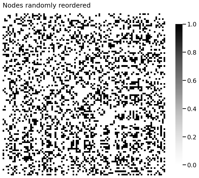
import numpy as np

# generate a reordering of the n nodes
permutation = np.random.choice(n, size=n, replace=False)

Aperm = A[permutation][:,permutation]
yperm = labels[permutation]
heatmap(Aperm, title="Nodes randomly reordered")

<Axes: title={'left': 'Nodes randomly reordered'}>

def ohe_comm_vec(z):
    """
    A function to generate the one-hot-encoded community
    assignment matrix from a community assignment vector.
    """
    K = len(np.unique(z))
    n = len(z)
    C = np.zeros((n, K))
    for i, zi in enumerate(z):
        C[i, zi - 1] = 1
    return C

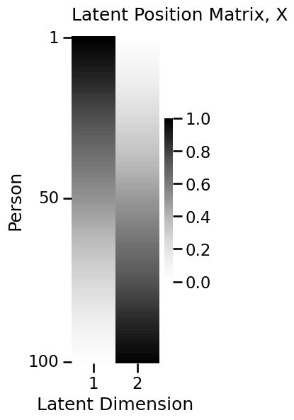
import numpy as np
from graphbook_code import lpm_heatmap

n = 100  # the number of nodes in our network
# design the latent position matrix X according to 
# the rules we laid out previously
X = np.zeros((n,2))
for i in range(0, n):
    X[i,:] = [(n - i)/n, i/n]

lpm_heatmap(X, ytitle="Person", xticks=[0.5, 1.5], xticklabels=[1, 2], 
            yticks=[0.5, 49.5, 99.5], yticklabels=[1, 50, 100],
            xtitle="Latent Dimension", title="Latent Position Matrix, X")

<Axes: title={'left': 'Latent Position Matrix, X'}, xlabel='Latent Dimension', ylabel='Person'>

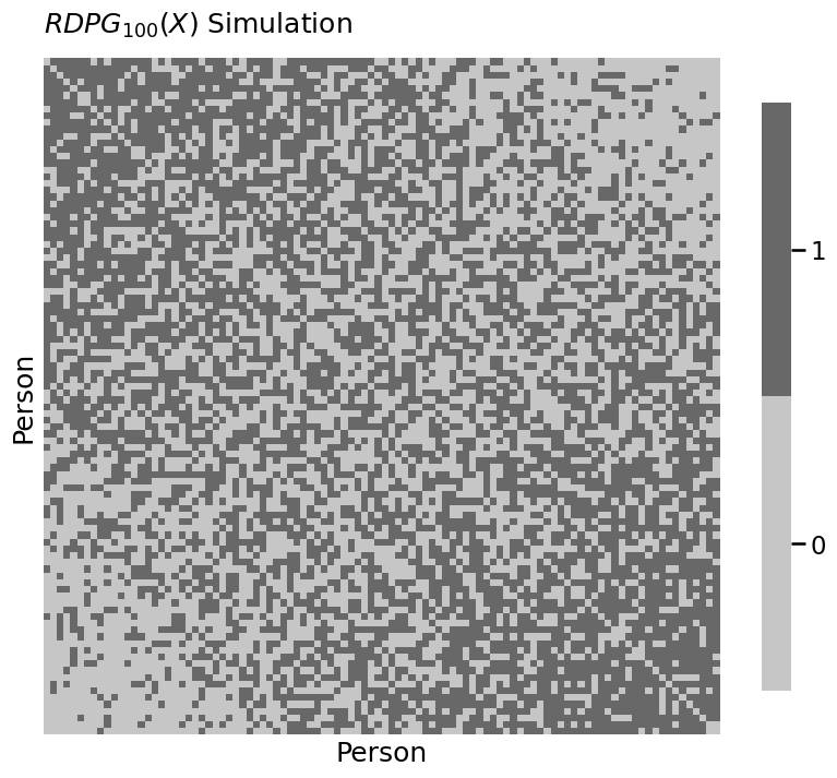
from graspologic.simulations import rdpg
from graphbook_code import heatmap

# sample an RDPG with the latent position matrix
# created above
A = rdpg(X, loops=False, directed=False)

# and plot it
heatmap(A.astype(int), xtitle="Person", ytitle="Person",
        title="$RDPG_{100}(X)$ Simulation")

<Axes: title={'left': '$RDPG_{100}(X)$ Simulation'}, xlabel='Person', ylabel='Person'>

import numpy as np

def block_mtx_psd(B):
    """
    A function which indicates whether a matrix
    B is positive semidefinite.
    """
    return np.all(np.linalg.eigvals(B) >= 0)

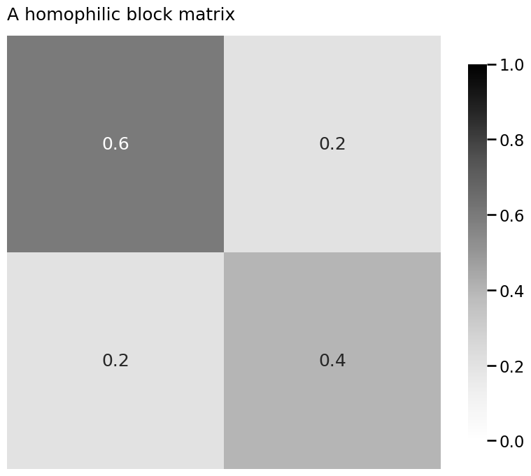
import numpy as np
from graphbook_code import heatmap

B = np.array([[0.6, 0.2], 
              [0.2, 0.4]])
heatmap(B, title="A homophilic block matrix", annot=True, vmin=0, vmax=1)
block_mtx_psd(B)
# True

True

B_indef = np.array([[.1, .2], 
                    [.2, .1]])
block_mtx_psd(B_indef)
# False

False

# a positive semidefinite kidney-egg block matrix
B_psd = np.array([[.6, .2], 
                  [.2, .2]])
block_mtx_psd(B_psd)
# True

# an indefinite kidney-egg block matrix
B_indef = np.array([[.1, .2], 
                    [.2, .2]])
block_mtx_psd(B_indef)
#False

False

# a positive semidefinite core-periphery block matrix
B_psd = np.array([[.6, .2], 
                  [.2, .1]])
block_mtx_psd(B_psd)
# True

# an indefinite core-periphery block matrix
B_indef = np.array([[.6, .2], 
                    [.2, .05]])
block_mtx_psd(B_indef)
# False

False

# an indefinite disassortative block matrix
B = np.array([[.1, .5], 
              [.5, .2]])
block_mtx_psd(B)
# False

False

# homophilic, and hence positive semidefinite, block matrix
B = np.array([[0.6, 0.2], 
              [0.2, 0.4]])

# generate square root matrix
sqrtB = np.linalg.cholesky(B)

# verify that the process worked through by equality element-wise
# use allclose instead of array_equal because of tiny
# numerical precision errors
np.allclose(sqrtB @ sqrtB.T, B)
# True

True

from graphbook_code import ohe_comm_vec

def lpm_from_sbm(z, B):
    """
    A function to produce a latent position matrix from a
    community assignment vector and a block matrix.
    """
    if not block_mtx_psd(B):
        raise ValueError("Latent position matrices require PSD block matrices!")
    # one-hot encode the community assignment vector
    C = ohe_comm_vec(z)
    # compute square root matrix
    sqrtB = np.linalg.cholesky(B)
    # X = C*sqrt(B)
    return C @ sqrtB

# make a community assignment vector for 25 nodes / community
nk = 25
z = np.repeat([1, 2], nk)

# latent position matrix for an equivalent RDPG
X = lpm_from_sbm(z, B)

from graphbook_code import generate_sbm_pmtx

# generate the probability matrices for an RDPG using X and SBM
P_rdpg = X @ X.T
P_sbm = generate_sbm_pmtx(z, B)

# verify equality element-wise
np.allclose(P_rdpg, P_sbm)
# True

True

import numpy as np
from graspologic.simulations import sample_edges
from graphbook_code import heatmap, plot_vector, \
    generate_sbm_pmtx

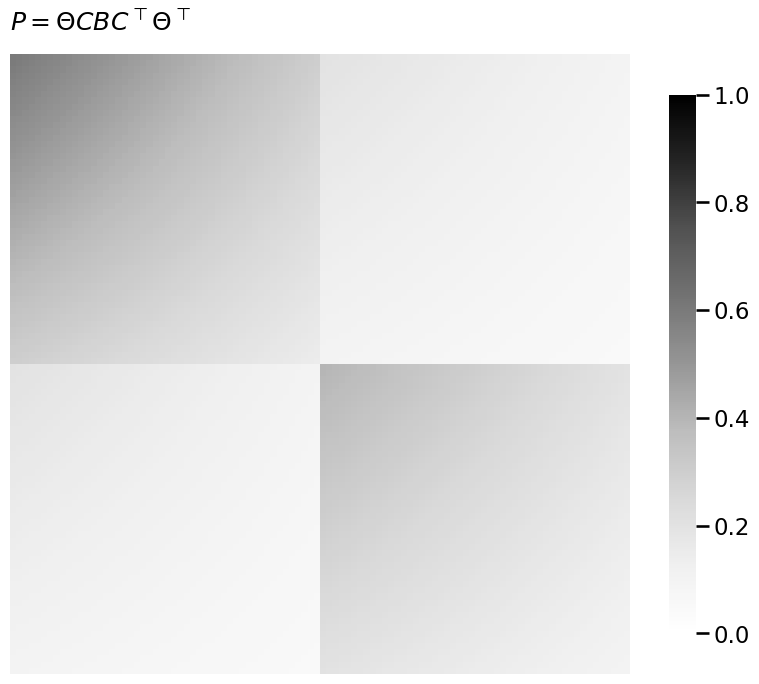
def dcsbm(z, theta, B, directed=False, loops=False, return_prob=False):
    """
    A function to sample a DCSBM.
    """
    # uncorrected probability matrix
    Pp = generate_sbm_pmtx(z, B)
    theta = theta.reshape(-1)
    # apply the degree correction
    Theta = np.diag(theta)
    P = Theta @ Pp @ Theta.transpose()
    network = sample_edges(P, directed=directed, loops=loops)
    if return_prob:
        network = (network, P)
    return network

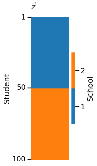
# Observe a network from a DCSBM
nk = 50  # students per school
z = np.repeat([1, 2], 50)
B = np.array([[0.6, 0.2], [0.2, 0.4]])  # same probabilities as from SBM section
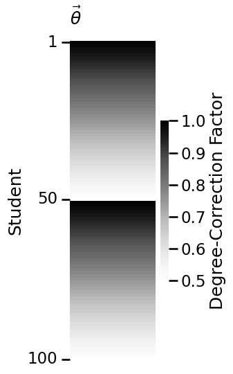
theta = np.tile(np.linspace(1, 0.5, nk), 2)
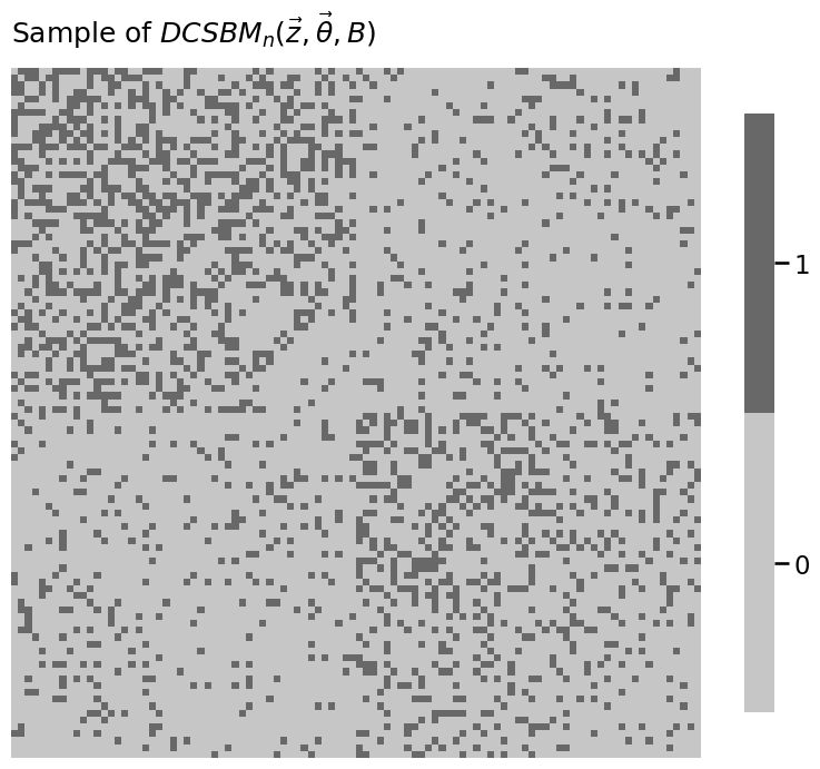
A, P = dcsbm(z, theta, B, return_prob=True)

# Visualize
plot_vector(z, title="$\\vec z$", legend_title="School", color="qualitative", 
            ticks=[0.5, 49.5, 99.5], ticklabels=[1, 50, 100],
            ticktitle="Student")
plot_vector(theta, title="$\\vec \\theta$", 
            legend_title="Degree-Correction Factor", 
            ticks=[0.5, 49.5, 99.5], ticklabels=[1, 50, 100],
            ticktitle="Student")
heatmap(P, title="$P = \\Theta C B C^\\top \\Theta^\\top$", vmin=0, vmax=1)
heatmap(A.astype(int), title="Sample of $DCSBM_n(\\vec z, \\vec \\theta, B)$")

<Axes: title={'left': 'Sample of $DCSBM_n(\\vec z, \\vec \\theta, B)$'}>

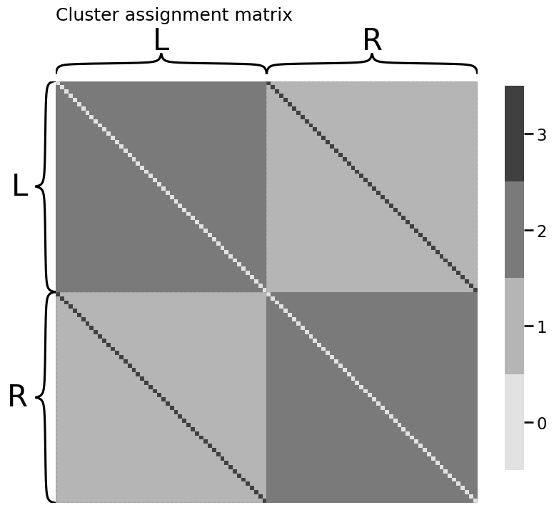
import numpy as np

n = 100
Z = np.ones((n, n))
for i in range(0, int(n / 2)):
    Z[int(i + n / 2), i] = 3
    Z[i, int(i + n / 2)] = 3
Z[0:50, 0:50] = Z[50:100, 50:100] = 2
np.fill_diagonal(Z, 0)

from graphbook_code import heatmap

labels = np.repeat(["L", "R"], repeats=n/2)
heatmap(Z.astype(int), title="Cluster assignment matrix", 
        inner_hier_labels=labels)

<Axes: title={'left': 'Cluster assignment matrix'}>

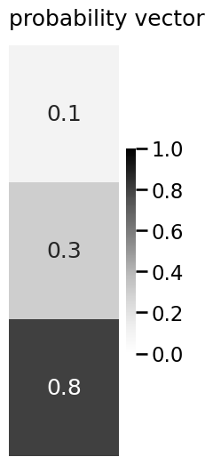
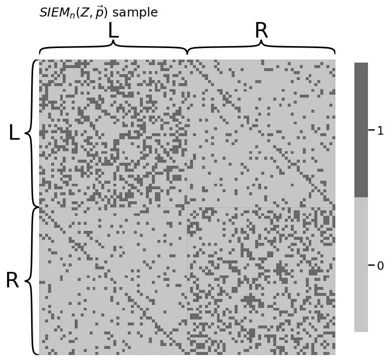
from graphbook_code import siem, plot_vector

p = np.array([0.1, 0.3, 0.8])
A = siem(n, p, Z)
plot_vector(p, title="probability vector", vmin=0, vmax=1, annot=True)
heatmap(A.astype(int), title="$SIEM_n(Z, \\vec p)$ sample", 
        inner_hier_labels=labels)

<Axes: title={'left': '$SIEM_n(Z, \\vec p)$ sample'}>

from graspologic.simulations import sbm
import numpy as np
from graphbook_code import dcsbm
from sklearn.preprocessing import LabelEncoder

# Create block probability matrix B
K = 3
B = np.full(shape=(K, K), fill_value=0.15)
np.fill_diagonal(B, 0.4)

# degree-correct the different groups for linkedin
ml, admin, marketing = nks = [50, 25, 25]
theta = np.ones((np.sum(nks), 1))
theta[(ml):(ml + admin), :] = np.sqrt(2)

# our dcsbm function only works with communities encoded 1,2,...,K
# so we'll use a LabelEncoder to map labels to natural numbers
labels = np.repeat(["ML", "AD", "MA"], nks)
le = LabelEncoder().fit(labels)
z = le.transform(labels) + 1

# sample the random networks
A_facebook = sbm(n=nks, p=B)
A_insta = sbm(n=nks, p=B)
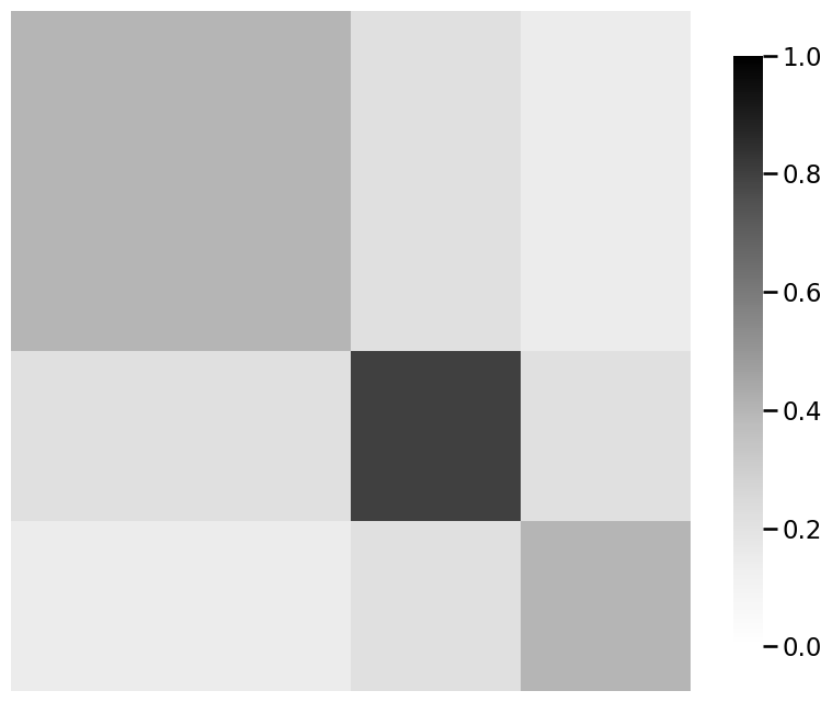
A_linkedin, P_linkedin = dcsbm(z, theta, B, return_prob=True)

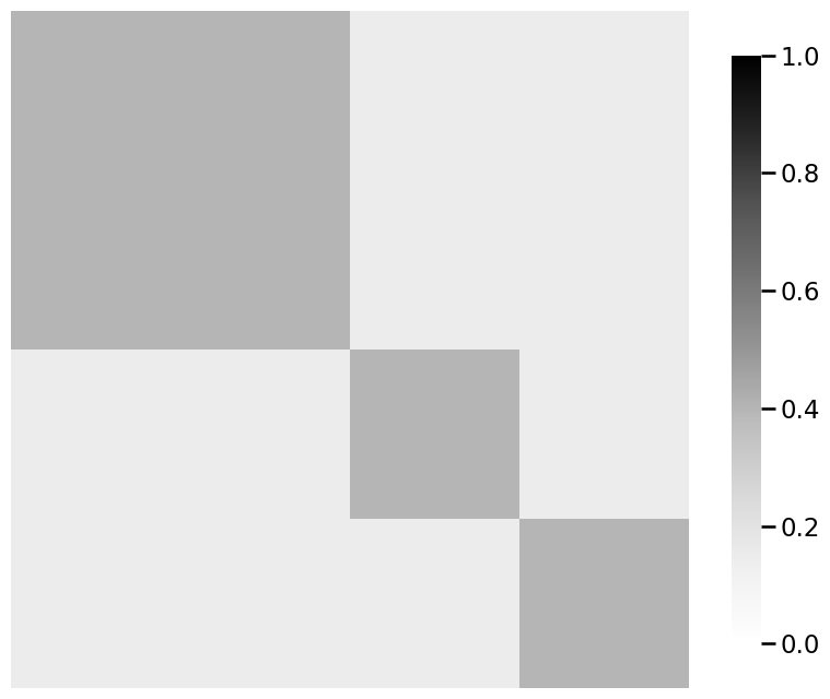
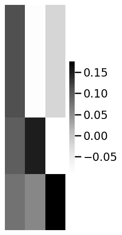
from graphbook_code import generate_sbm_pmtx, heatmap

# we already returned P_linkedin for the linkedin
# probability matrix from dcsbm() function
P_facebook_insta = generate_sbm_pmtx(z, B)

# when plotting for comparison purposes, make sure you are
# using the same scale from 0 to 1
heatmap(P_facebook_insta, vmin=0, vmax=1)
heatmap(P_linkedin, vmin=0, vmax=1)
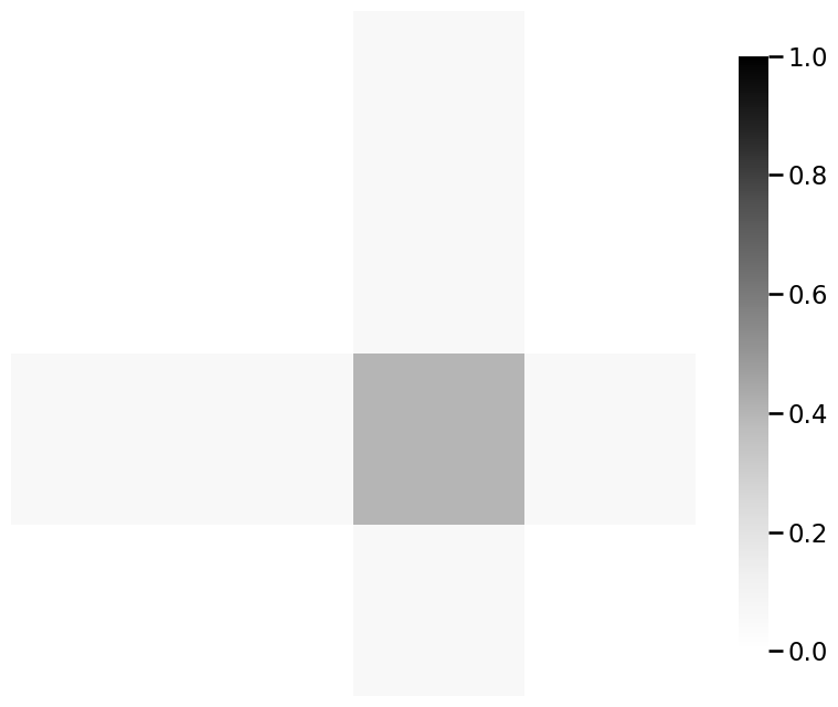
heatmap(P_linkedin - P_facebook_insta, vmin=0, vmax=1)

<Axes: >

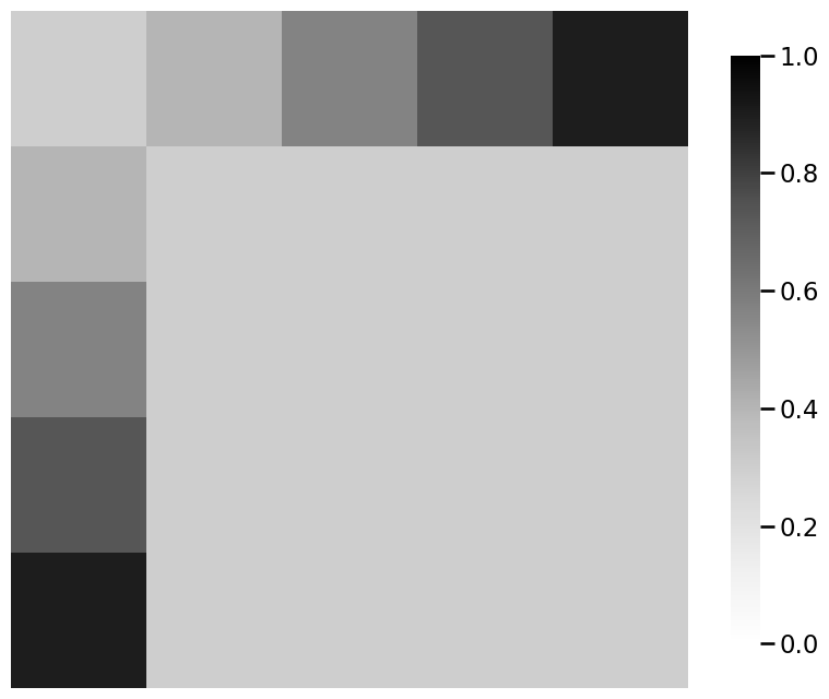
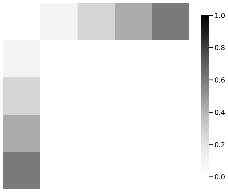
from graspologic.embed import MultipleASE as mase
from graphbook_code import lpm_heatmap

embedder = mase(n_components=3, svd_seed=0)
# obtain shared latent positions
S = embedder.fit_transform([P_facebook_insta, P_facebook_insta, P_linkedin])

lpm_heatmap(S)

<Axes: >

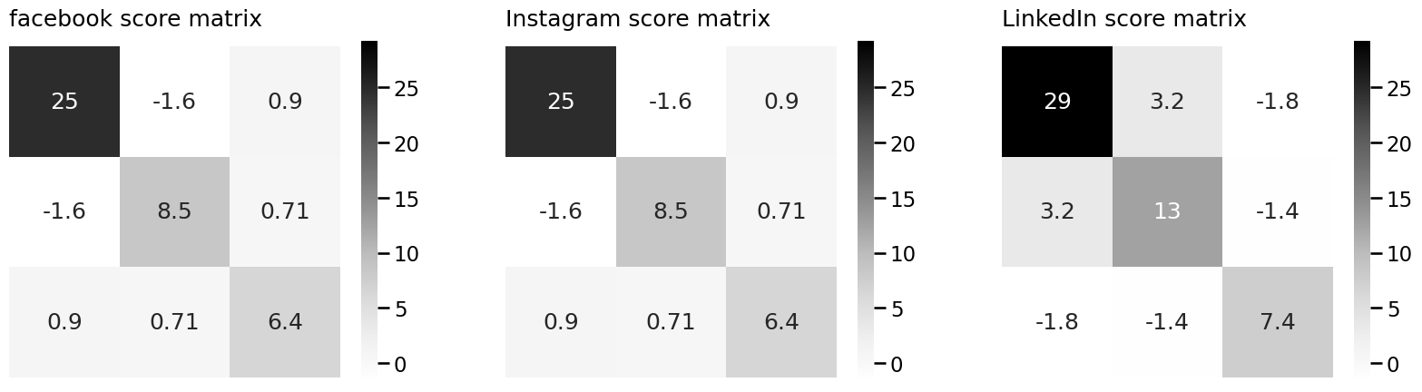
import matplotlib.pyplot as plt

R_facebook = embedder.scores_[0]
R_insta = embedder.scores_[1]
R_linkedin = embedder.scores_[2]

# and plot them
smin = np.min(embedder.scores_)
smax = np.max(embedder.scores_)

fig, axs = plt.subplots(1, 3, figsize=(20, 7))
heatmap(R_facebook, vmin=smin, vmax=smax, ax=axs[0], annot=True, title="facebook score matrix")
heatmap(R_insta, vmin=smin, vmax=smax, ax=axs[1], annot=True, title="Instagram score matrix")
heatmap(R_linkedin, vmin=smin, vmax=smax, ax=axs[2], annot=True, title="LinkedIn score matrix")

<Axes: title={'left': 'LinkedIn score matrix'}>

from graphbook_code import lpm_from_sbm
X_facebook_insta = lpm_from_sbm(z, B)

from graspologic.simulations import rdpg_corr

# generate the network samples
rho = 0.7
facebook_correlated_network, insta_correlated_network = rdpg_corr(
    X_facebook_insta, Y=None, r=rho
)

# the difference matrix
correlated_difference_matrix = np.abs(
    facebook_correlated_network - insta_correlated_network
)
# the total number of differences
correlated_differences = correlated_difference_matrix.sum()

rho_nil = 0.0
facebook_uncorrelated_network, insta_uncorrelated_network = rdpg_corr(
    X_facebook_insta, Y=None, r=rho_nil
)

# the difference matrix
uncorrelated_difference_matrix = np.abs(
    facebook_uncorrelated_network - insta_uncorrelated_network
)
# the total number of differences
uncorrelated_differences = uncorrelated_difference_matrix.sum()

import numpy as np
from graspologic.simulations import sample_edges

nodenames = [
    "SI", "L", "H/E", 
    "T/M", "BS"
]

# generate probability matrices
n = 5  # the number of nodes
P_earthling = 0.3*np.ones((n, n))
signal_subnetwork = np.zeros((n, n), dtype=bool)
signal_subnetwork[1:n, 0] = True
signal_subnetwork[0, 1:n] = True
P_astronaut = np.copy(P_earthling)
P_astronaut[signal_subnetwork] = np.tile(np.linspace(0.4, 0.9, num=4), 2)

# sample two networks
A_earthling = sample_edges(P_earthling)
A_astronaut = sample_edges(P_astronaut)

# plot probability matrices and their differences on the same scale
heatmap(P_earthling, vmin=0, vmax=1)
heatmap(P_astronaut, vmin=0, vmax=1)
heatmap(np.abs(P_astronaut - P_earthling), vmin=0, vmax=1)

<Axes: >

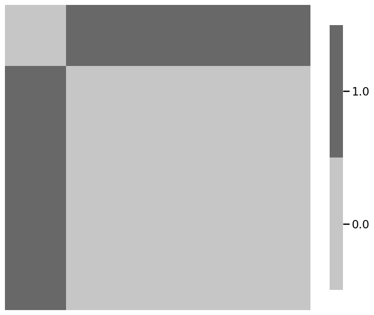
# plot the signal subnetwork
ax = heatmap(signal_subnetwork)

# sample the classes of each sample
M = 200  # the number of training and testing samples
pi_astronaut = 0.45
pi_earthling = 0.55
np.random.seed(0)
yvec = np.random.choice(2, p=[pi_earthling, pi_astronaut], size=M)

# sample network realizations given the class of each sample
Ps = [P_earthling, P_astronaut]

As = np.stack([sample_edges(Ps[y]) for y in yvec], axis=2)