2.3. Random Variables

2.3.1. Measurability

Next up is one of the most misunderstood (and most unnecessarily terrifying) concepts of traditional probability and statistics courses: the random variable. Let’s start with a definition:

Definition 2.38 (\((\mathcal F, \Sigma)\)-Random Variable)

Suppose that \((\Omega, \mathcal F)\) and \((S, \Sigma)\) are two measurable spaces. A function \(X : \Omega \rightarrow S\) is said to be a measurable map from \((\Omega, \mathcal F)\) to \((S, \Sigma)\) if for all \(B \in \Sigma\):

\[X^{-1}(B) \equiv \{X \in B\} \equiv \{\omega : X(\omega) \in B\} \in \mathcal F\]

Written another way:

\[X^{-1}(\Sigma) \equiv \{X^{-1}(B) : B \in \Sigma\} \equiv \left\{\{\omega : X(\omega) \in B\} : B \in \Sigma\right\}\subseteq \mathcal F\]

For such a measurable map \(X\), \(X\) is said to be a \((\mathcal F, \Sigma)\)-valued random variable, or it is \((\mathcal F, \Sigma)\)-measurable. In shorthand, we denote that \(X \in m(\mathcal F, \Sigma)\).

That definition was quite large, and the interpretation of this definition is really at the heart of the difference between traditional probability and statistics with measure theoretic probability and statistics. Let’s break down all of the things that this definition is saying.

The first aspect to fixate on here is that for some \(\omega \in \Omega\), \(X\) maps \(\omega\) to some other point \(s \in \mathcal S\).

All that the first line says is that, when we take some subset of the codomain \(S\) that is in the \(\sigma\)-algebra \(\Sigma\), \(B \in \Sigma\), that the set of all \(\omega\) where \(X(\omega) \in B\) is in the \(\sigma\)-algebra \(\mathcal F\) (this is made extremely clear by the right-most set). Stated mathematically, for any \(B \in \Sigma\), the preimage of \(B\) under \(X\) is a measurable set (it is in \(\mathcal F\)). The left two notations, \(X^{-1}(B)\) and \(\{X \in B\}\), are simply shorthands for the statement at the right. Random variables can, and will, become extremely confusing simply by way of people seeing the shorthands, and then forgetting what the shorthand actually means. The \(\equiv\) symbol is just used to make explicit that the notations are not just equal, they say exactly the same thing. The idea is that the preimage of elements of the \(\sigma\)-algebra of \(S\) are in the \(\sigma\)-algebra of \(\Omega\). So to work through this definition, let’s start by looking at \(X\) itself, which is just a function:

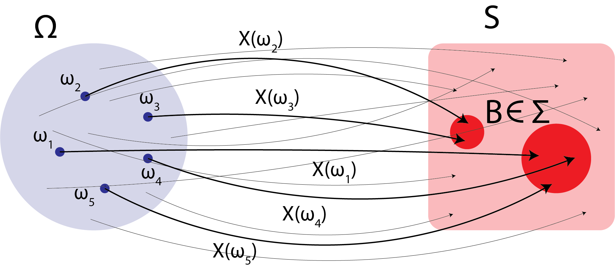
Fig. 2.7 Here, the blue circle represents individual elements \(\omega_i\) of the event space \(\Omega\), and the target space \(S\) is represented by the red square. For some \(B \in \Sigma\), represented by the red circles, there are a set of \(\omega\)s which are a subset of \(\Omega\) (and the set of such \(\omega\)s are in \(\mathcal F\)) that map to \(B\) under \(X\).

Now, let’s think about what the rest of those words mean in that definition, stated a (possibly more straightforward) way:

Remark 2.2 (Equivalent characterization for \((\mathcal F, \Sigma)\) random variable)

Suppose that \((\Omega, \mathcal F)\) and \((S, \Sigma)\) are two measurable spaces, and \(X \in m(\mathcal F, \Sigma)\). An equivalent interpretation of the definition of a random variable is that \(X^{-1} : \Sigma \rightarrow \mathcal F\).

This formulation is identical to Definition 2.38 and says it in a lot less words/math speak, and gives you a better idea regarding what’s going on. Further, as we’ll see later, use of this characterization will make proofs a little more obvious. So, all that’s happening here is that, for the elements of the sample space that got mapped to \(B \in \Sigma\), the preimage of the set \(B \in \Sigma\) under \(X\) (basically, the inverse), written \(X^{-1}(B)\), is the set of blue dots shown below:

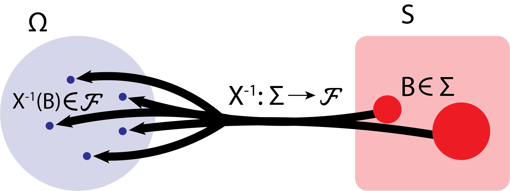
Fig. 2.8 Here, we instead start with the dark red circles, \(B\). The preimage of \(B\), \(X^{-1}(B)\), are the dark blue circles, and the set comprising the uniont of these dark blue circles is in \(\mathcal F\) (it is a measurable set).

All the notation going on here can get confusing, and while I’m going to take the time to write out the equivalences every time the first few times you see these sets arise in the remainder of this section, I’m going to (generally) shy away from that definition as the book progresses so that you can gradually get accustomed to the notation. Take a long hard look at the previous definition, the equivalent notations, and learn to love them!

Remark 2.3 (Shorthand when codomain is a subset of the reals)

Suppose that \((\Omega, \mathcal F)\) and \((S, \Sigma)\) are two measurable spaces, and \(X \in m(\mathcal F, \mathcal \Sigma)\). If \(S \subseteq \mathbb R\) and \(\Sigma = \mathcal B(S)\), then we will use the shorthand \(X \in m\mathcal F\).

Usually, the codomain are going to be real values, and the \(\sigma\)-algebra is just going to be the Borel \(\sigma\)-algebra, so it gets cumbersome to always have to write all of this out, so we adopt the above shorthand fairly often as the book proceeds.

There are some important consequences here.

Remark 2.4 (Discrete event space)

Suppose that the event space \(\Omega\) is discrete, and that \((\Omega, \mathcal F)\) is a measurable space. Then any \(X : \Omega \rightarrow \mathbb R\) is \(m\mathcal F\).

An important example of a random variable is the indicator random variable:

Example 2.12 (Indicator function)

Suppose that \((\Omega, \mathcal F)\) is a measurable space, and \(A \in \mathcal F\). Then the function:

\[\begin{split} \mathbb 1_{\{A\}}(\omega) &= \begin{cases} 1, & \omega \in A \\ 0, & \omega \not\in A \end{cases}\end{split}\]

is \(m\mathcal F\).

Finally, if it isn’t clear to you already, let’s just take a little step back and think about the word “random”:

Remark 2.5

You’ll often see us go back and forth throughout this book using the words measurable and random variable. Probability theorists tend to like the word random variable, and mathematicians tend to like the word measurable. We will tend to stick to the probability theory language later on, but it is important to cement in your head that there is nothing “random” about these things really; random variables (measurable functions), follow a prescribed set of rules, and really thinking hard about these rules will make them feel a little less mysterious.

2.3.2. Generators

Just like we could identify \(\sigma\)-algebras from generating sets, we can identify random variables from generating sets:

Theorem 2.4 (Random variable induced by generating sets)

Suppose that \((\Omega, \mathcal F)\) and \((S, \Sigma)\) are measurable spaces. that \(X : \Omega \rightarrow S\), and that \(\Sigma = \sigma(\mathcal A)\) for some family of subsets \(A \in \mathcal A\), where \(A \subseteq S\). Then if for all \(A \in \mathcal A\):

\[\begin{split} X^{-1}(A) = \{\omega : X(\omega) \in A\} &\in \mathcal F \\ \Rightarrow X^{-1}(\mathcal A) \subseteq \mathcal F\end{split}\]

\(X \in m(\mathcal F, \Sigma)\).

Proof. Let:

\[\begin{split}\mathcal B &\triangleq \{B \in \Sigma : X^{-1}(B) \in \mathcal F\} \\ &\equiv \mathcal B \triangleq \{B \in \Sigma : \{X \in B\} \in \mathcal F\} \\ &\equiv \mathcal B \triangleq \{B \in \Sigma : \{\omega : X(\omega) \in B\} \in \mathcal F\} \\ &\equiv X(\mathcal F)\end{split}\]

be a family of sets on \(S\), where \(\mathcal B\) are the subsets of the codomain \(S\) which land in \(\mathcal F\) under the inverse image of \(X\).

By construction, notice that \(X^{-1} : \mathcal B \rightarrow \mathcal F\).

To see that \(\mathcal B\) is a \(\sigma\)-algebra:

1. Contains \(\Omega\): Note that since \(X : \Omega \rightarrow S\), that for any \(\omega \in \Omega\), then \(X(\omega) \in S\).

Then since \(\Omega \in \mathcal F\), \(S \in \mathcal B\).

2. Closed under complements: Suppose that \(B \in \mathcal B\), so \(\{X \in B\}\equiv \{\omega : X(\omega) \in B\} \in \mathcal F\).

Further, note that \(\{\omega : X(\omega) \in B^c\} \equiv \{X \in B^c\} = \{X \in B\}^c \equiv \{\omega : X(\omega) \in B\}^c\), which follows because \(\{\omega : X(\omega) \in B\} = \Omega \setminus \{\omega : X(\omega) \in B^c\}\).

Then since \(\mathcal F\) is a \(\sigma\)-algebra where \(\{\omega : X(\omega) \in B\} \in \mathcal F\), then \(\{\omega : X(\omega) \in B\}^c \in \mathcal F\), since \(\mathcal F\) is closed under complement.

Then \(B^c \in \mathcal B\).

3. Closed under countable unions: Suppose that \(B_n \in \mathcal B\), where \(n \in \mathbb N\).

Then for all \(n \in \mathbb N\), \(\{X \in B_n\} \equiv \{\omega : X(\omega) \in B_n\} \in \mathcal F\).

Then since \(\mathcal F\) is closed under countable unions, \(\bigcup_{n \in \mathbb N}\{X \in B_n\} \in \mathcal F\).

Finally, note that \(\bigcup_{n \in \mathbb N}\{X \in B_n\} \equiv \bigcup_{n \in \mathbb N}\{\omega : X(\omega) \in B_n\}\) is identical to the set \(\left\{\omega : X(\omega) \in \bigcup_{n \in \mathbb N}B_n\right\} \equiv \left\{X \in \bigcup_{n \in \mathbb N}B_n \right\}\), so \(\left\{X \in \bigcup_{n \in \mathbb N}B_n \right\} \in \mathcal F\).

Then \(\bigcup_{n \in \mathbb N}B_n \in \mathcal B\).

Then by construction, \(X \in m(\mathcal F, \mathcal B)\).

Finally, we have to show that \(X\) is \(m(\mathcal F, \mathcal \Sigma)\).

By construction, \(\mathcal B \supseteq \mathcal A\), where \(\Sigma = \sigma(\mathcal A)\).

Then since \(\mathcal B\) is a \(\sigma\)-algebra that contains \(\mathcal A\), by Lemma 2.2, \(\mathcal B \supseteq \Sigma = \sigma(\mathcal A)\).

Then \(X^{-1} : \Sigma \rightarrow \mathcal F\).

Then \(X \in m(\mathcal F, \Sigma)\), by Remark 2.2.

Why is this result so important? As it turns out, establishing measurability of a function can be rather difficult. For instance, if the codomain is the real line \(\mathbb R\) and the \(\sigma\)-algebra is \(\mathcal R\), it might be really hard to establish that Definition 2.38 holds for every possible element of the \(\mathcal R\) (this, of course, being because describing \(\mathcal R\) in and of itself is tedious if not impossible). However, we can describe generators of \(\mathcal R\), and then we can use Theorem 2.4 to evaluate whether a function is measurable (a random variable).

Further, \(\sigma\)-algebras can be generated by random variables, as well:

Definition 2.39 (\(\sigma\)-algebra generated by random variable)

Suppose that \((\Omega, \mathcal F)\) and \((S, \Sigma)\) are measurable spaces. Then the \(\sigma\)-algebra generated by \(X \in m(\mathcal F, \Sigma)\) is:

\[\begin{split} \sigma(X) &\triangleq \{\{\omega : X(\omega) \in B\} : B \in \Sigma\} \equiv \{\{X \in B\} : B \in \Sigma\} \\ &\equiv \{X^{-1}(B) : B \in \Sigma\} = X^{-1}(\Sigma)\end{split}\]

Now that we have these two properties down, we’re going to take a look at how to use them in practice.

2.3.3. Elementary Operations

Random variables can do lots of interesting and useful things. One of the easiest to wrap your head around is composition:

Lemma 2.5 (Composition Lemma)

Suppose that \((\Omega, \mathcal F)\), \((S, \Sigma)\), and \((T, \mathcal T)\) are measurable spaces, where \(X \in m(\mathcal F, \Sigma)\) and \(f \in m(\Sigma, \mathcal T)\). Then \(f \circ X = f(X) \in m(\mathcal F, \mathcal T)\).

Proof. Recall that for \(f(X) \in m(\mathcal F, \mathcal T)\), that \((f\circ X)^{-1} : \mathcal T \rightarrow \mathcal F\).

Let \(B \in \mathcal T\).

Then:

\[\begin{split} \left\{(f\circ X)^{-1}(B)\right\} &\equiv \left\{\omega : (f\circ X)(\omega) \in B\right\} \\ &\equiv \left\{\omega : f(X(\omega)) \in B\right\},\,\,\,\,\text{defn. composition} \\ &= \left\{\omega : X(\omega) \in f^{-1}(B)\right\}\end{split}\]

Notice that with \(E = f^{-1}(B)\), that \(E \in \Sigma\), since \(f \in m(\Sigma, \mathcal T)\). Therefore:

\[\begin{split} \left\{(f\circ X)^{-1}(B)\right\} &= \left\{\omega : X(\omega) \in E\right\} \\ &= X^{-1}(E) \in \mathcal F\end{split}\]

which follows because \(X \in m(\mathcal \Sigma, \mathcal F)\).

Therefore \(f \circ X \in m(\mathcal F, \mathcal T)\).

2.3.3.1. Properties of Measurability

Also, measurability comes with some nice properties. First and foremost, the preimage of random variables preserve set unions and complements:

Property 2.11 (Measurable functions preserve elementary set operations)

Suppose that \((\Omega, \mathcal F)\) and \((\mathbb R, \mathcal R)\) are measurable spaces, and further suppose that Suppose that \(h : \Omega \rightarrow \mathbb R\), \(F_i \in \mathcal F\), for \(i \in \mathcal I\). Then \(h^{-1}\) preserves elementary set operations; that is:

\[h^{-1}\left(\bigcup_{i \in \mathcal I} F_i\right) = \bigcup_{i \in \mathcal I}h^{-1}(F_i)\;\text{ and }\;h^{-1}(F_i^c) = \left(h^{-1}(F_i)\right)^c\]

Proof. 1. Unions:

\[\begin{split}h^{-1}\left(\bigcup_{i \in \mathcal I} F_i\right) &= \left\{\omega : h(\omega) \in \bigcup_{i \in \mathcal I} F_i\right\},\,\,\,\,\text{defn. preimage} \\ &= \left\{ \omega : \exists i \in \mathcal I : h(\omega) \in F_i\right\},\,\,\,\,\text{defn. union} \\ &= \bigcup_{i \in \mathcal I}\{\omega : h(\omega) \in F_i\} \\ &= \bigcup_{i \in \mathcal I}h^{-1}(F_i)\end{split}\]

2. Complements:

\[\begin{split}h^{-1}(F_i^c) &= \{\omega : h(\omega) \in F_i^c\} \\ &= \{\omega : h(\omega) \not\in F_i\} \\ &= \Omega \setminus \{\omega : h(\omega) \in F_i\} \equiv \{\omega : h(\omega) \in F_i\}^c \\ &= \left(h^{-1}(F_i)\right)^c\end{split}\]

Next, we’ll see how continuity and measurability go hand-in-hand:

Property 2.12 (Continuity implies measurability)

Suppose that \((\Omega, \mathcal F)\) and \((\mathbb R, \mathcal R)\) are measurable spaces, and suppose that \(h : \Omega \rightarrow \mathbb R\) is continuous. Then \(h \in m(\mathcal B(\Omega), \mathcal R)\).

Proof. Recall that \(\mathcal B(\Omega) \triangleq \sigma(\{\text{open sets on }\Omega\})\).

Let \(\mathcal C = \{\text{open sets on }\mathbb R\}\), where by definition, \(\mathcal R = \sigma(\mathcal C)\).

Since \(h : \Omega \rightarrow \mathbb R\) is continuous, then \(h^{-1}(C)\) for \(c \in \mathcal C\) is an open set \(B\) in \(\Omega\). This follows since \(C\) is open, and the preimage of continuous functions on open sets is open.

Then \(B \subseteq \mathcal B(\Omega)\), for every \(C \in \mathcal C\).

Then \(X^{-1} : \mathcal C \rightarrow \mathcal B(\Omega)\), so by Theorem 2.4, \(X^{-1} : \sigma(\mathcal C) = \mathcal R \rightarrow \mathcal B(\Omega)\), and \(X \in m(\mathcal B(\Omega), \mathcal R)\).

This means that if a function is continuous from \(\Omega\) to \(\mathbb R\), it is a \((\mathcal B(\Omega), \mathcal R)\) random variable.

Finally, we’ll see an extremely useful corollary of Theorem 2.4 when the codomain is \(\mathbb R\) and the \(\sigma\)-algebra is \(\mathcal R\). This corollary will make proving measurability quite easy for some sets of functions:

Corollary 2.1 (Generator sets of \(\mathcal R\))

Suppose that \((\Omega, \mathcal F)\) and \((\mathbb R, \mathcal R)\) are measurable spaces. Then \(h \in m(\mathcal F, \mathcal R) \iff \{h \leq \lambda\} \in m(\mathcal F, \mathcal R)\) for any \(\lambda \in \mathbb R\).

Proof. 1. Suppose that \(h \in m(\mathcal F, \mathcal R)\).

Recall that sets of the form \((-\infty, r] \in \mathcal R\), since \(\{(-\infty, r] : r \in \mathbb R\}\) is a generator of \(\mathbb R\).

Then \(h^{-1}(-\infty, r] \equiv \{h \leq r\} \in \mathcal F\).

2. Suppose that \(\{h \leq \lambda\} \in \mathcal F\), for any \(\lambda \in \mathbb R\).

Let \(\mathcal C = \{(-\infty, \lambda] : \lambda \in \mathbb R\}\) be another generator of \(\mathcal R\).

Then note that by supposition that \(\{h \leq \lambda\} \equiv h^{-1}(-\infty, \lambda] \in \mathcal F\), so for any \(C \in \mathcal C\), \(h^{-1}(C) \in \mathcal F\).

Then by Theorem 2.4, \(h \in m(\mathcal F, \mathcal R)\).

Pretty neat, right? So, when the codomain is \(\mathbb R\), all we need to do is prove it on generator sets. In the other direction, we also obtain that if we have a random variable, we can determine inequalities about it, which we’ll use later on extensively.

Remark 2.6

It is not hard to conceptualize that we can use this property to deduce all of the other inequalities as well, by chaining this result together with Property 2.12 and using properties about \(\sigma\)-algebras (closures under complements, countable intersections, countable unions, and containing the event space). Let’s see how we can use it now. Note that we might refer back to this theorem with other generator sets, but you should have in your head that the process/intuitition is the same across all of these results.

2.3.3.2. Mathematical Operations

If we want to be able to use random variables, it would be extremely convenient if we could add, multiply, and rescale them. We’ll formalize these operations now, which if you take notice, will all be trivial applications of Corollary 2.1 like we just discussed:

Property 2.13 (Addition of random variables)

Suppose that \((\Omega, \mathcal F)\) and \((\mathbb R, \mathcal R)\) are measurable spaces, and that \(X_1, X_2 \in m(\mathcal F, \mathcal R) : \Omega \rightarrow \mathbb R\). Then \(X_1 + X_2 \in m(\mathcal F, \mathcal R)\).

Proof. Denote \(Y = X_1 + X_2 \equiv Y(\omega) = X_1(\omega) + X_2(\omega)\).

By Corollary 2.1, it suffices to show that for every \(r \in \mathbb R\), that \(\{Y \leq r\} \equiv \{\omega : Y(\omega) \leq r\} \in \mathcal F\).

Note that:

\[\begin{split} \{Y \leq r\} &= \{X_1 + X_2 \leq r\} \\ &= \{X_1 \leq r - X_2\} \\ &= \{X_1 > r - X_2\}^c \\ &= \{X_1 > q > r - X_2\}^c,\,\,\,\, q \in \mathbb Q\end{split}\]

This result follows because, if \(X_1(\omega), r - X_2(\omega) \in \mathbb R\), then \(\exists q \in \mathbb Q\) s.t. \(q \in (X_1(\omega), r - X_2(\omega))\).

Continuing, and noting that the existence of such a \(\mathbb Q\) implies that we can take the (countable, as \(\mathbb Q\) is countably infinite) union of all of these such sets:

\[\begin{split} \{Y \leq r\} &= \left(\bigcup_{q \in \mathbb Q}\{X_1 > q > r - X_2\}\right)^c \\ \{Y \leq r\} &= \left(\bigcup_{q \in \mathbb Q}\{X_1 > q\} \cap \{q > r - X_2\}\right)^c\end{split}\]

Remember that \(\mathcal F\) is a \(\sigma\)-algebra, so since \(X_1, X_2 \in m(\mathcal F, \mathcal R)\), then \(\{X_1 > q\}, \{q > r - X_2\} \equiv \{X_2 > r - q\}\), their finite intersection, the countable union, and the complement are also in \(\mathcal F\), because \(\sigma\)-algebras are closed under all of these operations.

Then \(\{Y \leq r\} \in \mathcal F\).

Then by Corollary 2.1, \(Y = X_1 + X_2 \in m(\mathcal F, \mathcal R)\).

Property 2.14 (Multiplication of random variables)

Suppose that \((\Omega, \mathcal F)\) and \((\mathbb R, \mathcal R)\) are measurable spaces, and that \(X_1, X_2 \in m(\mathcal F, \mathcal R) : \Omega \rightarrow \mathbb R\). Then \(X_1 + X_2 \in m(\mathcal F, \mathcal R)\).

Proof. Denote \(Y = X_1 \cdot X_2 \equiv Y(\omega) = X_1(\omega)X_2(\omega)\).

By Corollary 2.1 and Property 2.11, it suffices to show that for every \(r \in \mathbb R\), that \(\{Y > r\} \equiv \{\omega : Y(\omega) > r\} \in \mathcal F\).

Suppose WOLOG that \(X_1, X_2\) are s.t. \(X_1(\omega), X_2(\omega) \geq 0\) for all \(\omega \in \Omega\).

Note that for all \(r \in \mathbb R_{< 0}\), that:

\[ \{\omega \in \Omega : X_1(\omega)X_2(\omega) > r\} = \Omega \in \mathcal F\]

since \(\mathcal F\) is a \(\sigma\)-algebra and must contain the event space.

If \(r \geq 0\), then:

\[\begin{split} \{\omega \in \Omega : X_1(\omega)X_2(\omega) > r\} &= \bigcup_{q \in \mathbb Q_{> 0}}\left\{\omega \in \Omega : X_1(\omega) > q, X_2(\omega) > \frac{r}{q}\right\} \\ &= \bigcup_{q \in \mathbb Q_{> 0}}\left(\left\{\omega \in \Omega : X_1(\omega) > q\right\}\cap \left\{\omega \in \Omega : X_2(\omega) > \frac{r}{q}\right\}\right) \\ &\in \mathcal F\end{split}\]

Which follows because \(\mathcal F\) is a \(\sigma\)-algebra, and hence closed under countable unions and finite intersections in \(\mathcal F\).

Then by Corollary 2.1, \(Y = X_1 \cdot X_2 \in m(\mathcal F, \mathcal R)\).

In the preceding proof, we made our lives a lot easier with the WOLOG statement; you could also repeat (nearly) same argument, going case-by-case, for the cases where \(X_1(\omega) < 0\) but \(X_2(\omega) \geq 0\), so on and so-forth.

Property 2.15 (Rescaling of random variables)

Suppose that \((\Omega, \mathcal F)\) and \((\mathbb R, \mathcal R)\) are measurable spaces, that \(X \in m(\mathcal F, \mathcal R) : \Omega \rightarrow \mathbb R\), and \(\lambda \in \mathbb R\). Then \(\lambda X \in m(\mathcal F, \mathcal R)\).

Proof. If \(\lambda = 0\), then for any \(r \in \mathbb R\):

\[ \{\omega \in \Omega : \lambda X(\omega) > r\} = \{\omega \in \Omega : 0 > r\} \in \{\Omega, \varnothing\} \in \mathcal F,\]

since \(\mathcal F\) is a \(\sigma\)-algebra (and hence contains the event space \(\Omega\) and its complement, the empty set \(\varnothing\)).

If \(\lambda \neq 0\), then for \(r \in \mathbb R\):

\[\begin{split} \{\omega \in \Omega : \lambda X(\omega) > r\} &= \begin{cases} \{\omega \in \Omega : X(\omega) > \frac{r}{\lambda}\}, & \lambda > 0 \\ \{\omega \in \Omega : X(\omega) < \frac{r}{\lambda}\}, & \lambda < 0 \end{cases} \in \mathcal F\end{split}\]

which follows by Corollary 2.1 and Property 2.11.

Then by Corollary 2.1, \(Y = \lambda X \in m(\mathcal F, \mathcal R)\).

2.3.3.3. Measurable limits and extrema

I’d recommend that you take a look back at Section 2.1.6 for a quick recap of set-theoretic limits before proceeding with this next section since we haven’t quite used these ideas all that much thus far. Let’s see how this works:

Property 2.16 (Infimum is measurable)

Suppose that \(X_n \in m(\mathcal F, \mathcal R) : \Omega \rightarrow \mathbb R\), for \(n \in \mathbb N\), where \((\Omega, \mathcal F)\) and \((\mathbb R, \mathcal R)\) are measurable spaces. Then \(Y = \inf_n X_n \in m(\mathcal F, \mathcal R)\).

Proof. Suppose that \(r \in \mathbb R\).

Recall that with \(Y = \inf_n X_n\), that if \(\omega \in \Omega\), \(Y(\omega) \geq r\) if for all \(n \in \mathbb N\), \(X_n(\omega) \geq r\), by definition of an infimum.

Then:

\[\begin{split} \{\omega : Y(\omega) \geq r\} &= \left\{\omega : \left(\inf_n X_n\right)(\omega) \geq r\right\} \\ &= \bigcap_n \left\{\omega : X_n(\omega) \geq r\right\},\,\,\,\, Y \geq r \iff \forall n,\, X_n \geq r \\ &= \bigcap_n \{X_n \geq r\} \\ &\in \mathcal F\end{split}\]

Which follows because \(X_n \in m(\mathcal F, \mathcal R)\), so \(\{X_n \geq r\} \in \mathcal F\) by Corollary 2.1, and \(\mathcal F\) is closed under countable intersections.

Then by Corollary 2.1, \(Y \in m(\mathcal F, \mathcal R)\).

This theorem asserts that the infimum of a sequence \(\{X_n\}\) of random variables is a random variable, too. The same holds for the supremum:

Property 2.17 (Supremum is measurable)

Suppose that \(X_n \in m(\mathcal F, \mathcal R) : \Omega \rightarrow \mathbb R\), for \(n \in \mathbb N\), where \((\Omega, \mathcal F)\) and \((\mathbb R, \mathcal R)\) are measurable spaces. Then \(Y = \sup_n X_n \in m(\mathcal F, \mathcal R)\).

Proof. Suppose that \(r \in \mathbb R\).

Recall that with \(Y = \sup_n X_n\), that with \(\omega \in \Omega\), \(Y(\omega) \leq r\) if for all \(n \in \mathbb N\), \(X_n(\omega) \leq r\), by definition of a supremum.

Proceed with the same argument to Property 2.16, instead using the sets \(\{X_n \leq r\}\) in the intersections.

Further, the \(\liminf\) and \(\limsup\) are random variables, too:

Theorem 2.5 (\(\liminf\) is measurable)

Suppose that \(X_n \in m(\mathcal F, \mathcal R) : \Omega \rightarrow \mathbb R\), for \(n \in \mathbb N\), where \((\Omega, \mathcal F)\) and \((\mathbb R, \mathcal R)\) are measurable spaces. Then \(Y = \liminf_n X_n \in m(\mathcal F, \mathcal R)\).

Proof. Recall that \(\liminf_n X_n \equiv \sup_n \inf_{m \geq n} X_n\), and define \(Y_n = \inf_{m \geq n} X_n\).

Notice that \(Y_n \in m(\mathcal F, \mathcal R)\), by Property 2.16.

Then \(Y = \sup_n Y_n \in m(\mathcal F, \mathcal R)\), by Property 2.17.

Property 2.18 (\(\limsup\) is measurable)

Suppose that \(X_n \in m(\mathcal F, \mathcal R) : \Omega \rightarrow \mathbb R\), for \(n \in \mathbb N\), where \((\Omega, \mathcal F)\) and \((\mathbb R, \mathcal R)\) are measurable spaces. Then \(Y = \limsup_n X_n \in m(\mathcal F, \mathcal R)\).

Proof. Recall that \(\limsup_n X_n \equiv \inf_n \sup_{m \geq n} X_n\), and define \(Y_n = \sup_{m \geq n} X_n\).

Notice that \(Y_n \in m(\mathcal F, \mathcal R)\), by Property 2.17.

Then \(Y = \sup_n Y_n \in m(\mathcal F, \mathcal R)\), by Property 2.16.