2.2. Measures#
The main reason that \(\sigma\)-algebras are powerful for our field of study is that they are special mathematical objects to which we can assign something called a measure. To do this, we’ll build towards measures, first starting with set functions, which allow us to ascribe units to families of sets like algebras.
2.2.1. Set functions#
Set functions are the basic building blocks we need to define measures. In effect, set functions allow us to ascribe some notion of size to sets in algebras:
Definition 2.21 (Set function)
Suppose that \(\Omega\) is a set, and let \(\mathcal A\) be an algebra on \(\Omega\). \(\mu_0\) is called a set function if \(\mu_0 : \mathcal A \rightarrow \bar{\mathbb R}_{\geq 0}\).
The space \(\bar{\mathbb R}\) is called the extended real numbers, which just means that it includes \(\infty\) and \(-\infty\). The subscript \(\geq 0\) just delineates that it is the non-negative component. Written another way, \(\bar{\mathbb R}_{\geq 0} = [0, \infty]\).
Just like algebras were closed under particular operations (finitely many unions), set functions have analogous operations, too. However, it is important to recognize that set functions need not have the below listed properties, which is why these types of set functions have special names:
Definition 2.22 (Additive set function)
Suppose that \(\Omega\) is a set, and let \(\mathcal A\) be an algebra on \(\Omega\). \(\mu_0\) is called an additive set function if:
\(\mu_0(\varnothing) = 0\), and
if \(A_1, A_2 \in \mathcal A\) are s.t. \(A_1 \cap A_2 = \varnothing\) (they are disjoint), then \(\mu_0(A_1 \sqcup A_2) = \mu_0(A_1) + \mu_0(A_2)\).
We can show that this property extends to finitely many operations, too:
Example 2.10
Suppose that \(\Omega\) is a set, and let \(\mathcal A\) be an algebra on \(\Omega\). Show that if \(\mu_0\) is an additive set function, then if \(A_m \in \mathcal A\) are mutually disjoint for \(m \in [n]\) where \(n \in \mathbb N\), that:
Let’s see an example of this, with a figure:
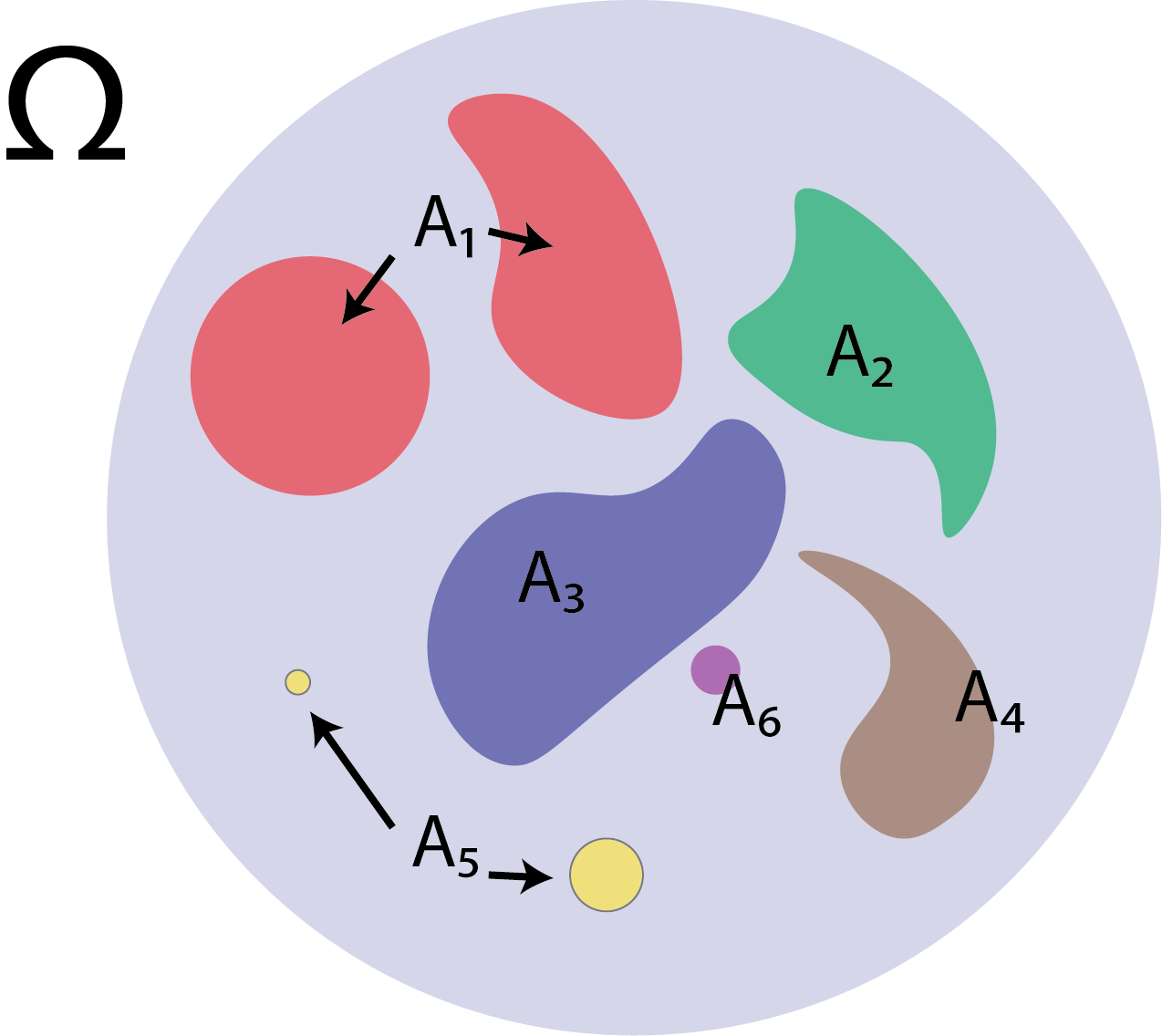
Fig. 2.2 Here, we show the sample space \(\Omega\) in blue. In this and succeeding figures, you can conceptualize the measure of a set to be its area (e.g., this example shows a finite measure, since \(\mu(\Omega) < \infty\)). The sets \(A_i\) are the shapes shown, where each \(A_i\) has a different color. Notice, in particular, that the sets are disjoint, in that they are not overlapping. If we wanted to measure (compute the area, in this context) of the union of such disjoint sets, the measure of the area of all of these disjoint objects would just be the sum of the area of each disjoint object individually (e.g., compute the area of each shaded region corresponding to an \(A_i\), and then sum them up).#
Countably additive set functions extend this property from finitely many operations to countably many operations:
Definition 2.23 (Countably additive set function)
Suppose that \(\Omega\) is a set, and let \(\mathcal A\) be an algebra on \(\Omega\). \(\mu_0\) is called a countably additive set function if:
\(\mu_0(\varnothing) = 0\), and
if \((A_n)_{n \in \mathbb N} \subseteq \mathcal A\) are a sequence of mutually disjoint sets, then:
It should be pretty obvious to you that a countably additive set function is additive:
Example 2.11
Suppose that \(\Omega\) is a set, and let \(\mathcal A\) be an algebra on \(\Omega\). Show that if \(\mu_0\) is a countably additive set function, it is also additive.
2.2.2. Measures#
Now that we have countably additive set functions, we are ready to wrap our heads around one of the most crucial topics that we will discuss so far: measures. The event space (and a \(\sigma\)-algebra defined on it) are called a measurable space:
Definition 2.24 (Measurable Space \((\Omega, \mathcal F)\))
The tuple \((\Omega, \mathcal F)\) is called a measurable space, if:
\(\Omega\) is a set,
\(\mathcal F\) is a \(\sigma\)-algebra on \(\Omega\).
A measure, in effect, allows us to formalize the concept of relational size, and unite it with what we’ve learned so far about countably additive set functions:
Definition 2.25 (Measure \(\mu\))
Let \((\Omega, \mathcal F)\) be a measurable space. A measure \(\mu : \mathcal F \rightarrow \bar{\mathbb R}_{\geq 0}\) is a non-negative countably additive set function, where:
Measure of empty set is zero: \(\mu(\varnothing) = 0\),
Non-negative: For any \(F \in \mathcal F\), \(\mu(F) \geq 0\),
Countably additive: If \(\{F_i\}_{i \in \mathbb N} \subseteq \mathcal F\) is a countable sequence of disjoint events, then:
The idea here is that, as we stated, set functions allow us to ascribe a notion of size to countably additive subsets of the algebra \(\mathcal A\). However, since an algebra is closed under only finitely many unions, we have no idea whether the resulting thing we ascribed size to even makes sense with respect to the algebra (it only necessarily holds meaning with respect to the space upon which the algebra was defined, \(\Omega\)). However, the measure defined on a measurable space ascribes size to countable unions of mutually disjoint subsets of \(\mathcal F\) (which is a \(\sigma\)-algebra). Therefore, this countable union of mutually disjoint subsets will actually end up being meaningful with respect to the measurable space (since the resulting countable union will also be contained in \(\mathcal F\), since \(\sigma\)-algebras are closed under countable unions).
By the second property, we obtain the logic of why we call \((\Omega, \mathcal F)\) a measurable space: it ascribes measure to measurable sets:
Definition 2.26 (Measurable set)
Suppose that \((\Omega, \mathcal F)\) is a measurable space. Then every \(F \in \mathcal F\) is called a measurable set.
The idea is measures ascribe reasonable notions of size to the measurable sets. When you read through Section 2.1, any time you see a result that concerns a \(\sigma\)-algebra being closed under something (e.g., countable unions, extrema, limits) you can say that these properties produce sets which are measurable if the sets they perform operations on are measurable.
Due to the fact that these two concepts of a measurable space and a measure are so complementary in this regard (one provides a set and a family of measurable sets, the other prescribes a function for ascribing relational size to the measurable sets), we often group these ideas together with the word measure space:
Definition 2.27 (Measure Space \((\Omega, \mathcal F, \mu)\))
The triple \((\Omega, \mathcal F, \mu)\) is called a measure space if:
\(\Omega\) is a set,
\(\mathcal F\) is a \(\sigma\)-algebra on \(\Omega\), and
\(\mu : \mathcal F \rightarrow \mathbb R\) is a measure on \((\Omega, \mathcal F)\).
You’ll notice that the only restriction we placed on measures were that they were non-negative. This means that \(\mu : \mathcal F \rightarrow \bar{\mathbb R}_{\geq 0}\), which means that we could, feasibly, have some sets with infinite measures. This theoretical note tends to not be particularly nice for our field of study, so we’ll introduce two related types of measures which remove this oddity:
Definition 2.28 (Finite measure space)
Suppose that \((\Omega, \mathcal F, \mu)\) is a measure space. The measure space, and the measure \(\mu\), are called finite if \(\mu(\Omega) < \infty\).
As a consequence here, \(\mu : \mathcal F \rightarrow \mathbb R_{\geq 0}\), non-inclusive of \(\infty\). When you think about the properties of measures below, start to think about why the restriction that \(\mu(\Omega) < \infty\) implies that for any \(F \in \mathcal F\), \(\mu(F) < \infty\) for a finite measure.
This definition, unfortunately, tends to be a little bit restrictive, for a reason that you’ll see in an exercise later on. For this reason, we can “tweak” this definition a little bit, and instead define measure spaces that are finite only for the sets we actually care about: subsets of the \(\sigma\)-algebra. This gives us the concept of a \(\sigma\)-finite measure space:
Definition 2.29 (\(\sigma\)-finite measure space)
Suppose that \((\Omega, \mathcal F, \mu)\) is a measure space. The measure space, and the measure \(\mu\), are called \(\sigma\)-finite if there exists a sequence \((S_n)_{n \in \mathbb N} \subseteq \mathcal F\), s.t.:
For all \(F_n\), \(\mu(F_n) < \infty\), and
\(\bigcup_{n \in \mathbb N}F_n = \Omega\).
With this definition, we can still have \(\mu(\Omega) = \infty\), but we can still define countable sequences where each element has finite measure that unite to \(\Omega\). This may feel kind of like an edge-case situation, but it is going to be ultra necessary any time we try to deal with spaces that are uncountably infinite such as \(\mathbb R\).
2.2.2.1. Properties of measures#
In this book, we will often use (and abuse) several basic properties of measures. We’ll go through some of these now. To start off, we have the monotonicity of measures:
Property 2.3 (Monotonicity of measures)
Let \((\Omega, \mathcal F, \mu)\) be a measure space. Then if \(F_1 \subseteq F_2\) and \(F_1, F_2 \in \mathcal F\), \(\mu(F_1) \leq \mu(F_2)\).
Proof. Let \(F_1, F_2 \in \mathcal F\), where \(F_1 \subseteq F_2\).
Recall that \(F_2 \setminus F_1 = F_2 \cap F_1^c\). This represents the elements of \(F_2\) that are not in \(F_1\), so we could alternatively express \(F_2 = F_1 \cup (F_2 \setminus F_1)\).
As \(F_2 \setminus F_1\) is disjoint from \(F_1\):
as desired.
Intuitively, what this statement asserts is that the measure of a set which comprises another set must be at least the measure of the set it comprises. Let’s take a look at a picture which explains what’s going on:

Fig. 2.3 Again, we show the sample space \(\Omega\) in blue. Here, the \(F_2\) (in red) \(\supseteq F_1\) (in blue; since it is contained within \(F_2\), it looks purple). Notice that in this case, the measure (the area) \(\mu(F_2) \geq \mu(F_1)\).#
This concept extends to the case when \(A\) is a subset of a countable union of sets as well, and is called subadditivity:
Property 2.4 (Subadditivity of measures)
Let \((\Omega, \mathcal F, \mu)\) be a measure space. If \(F \subseteq \bigcup_{n \in \mathbb N}F_n\) where \(F, F_n \in \mathcal F\) for all \(n \in \mathbb N\), then:
Proof. Let \(F_n' = F_n \cap F\), for all \(n \in \mathbb N\). Like above, \(F_n'\) are the elements of \(F_n\) that are also in \(F\).
Define \(A_1 = F_1'\), and let \(A_n = F_n' \setminus \bigcup_{m = 1}^{n - 1}F_m'\) for all \(n > 1\). \(A_n\) represents the elements of \(F_n\) that are in \(F\), but are not in any of the preceding sets \(A_m\) where \(m \leq n\).
Note that \(A_n\) are disjoint by construction, since each set adds only the unique elements of \(F_n\) in \(F\) that are not in any of the preceding sets \(A_m\), and that \(F = \bigsqcup_{n \in \mathbb N}A_n\).
Further, note that \(A_n \subseteq F_n\), so:
which follows by Property 2.3.
This proof is a little tough, so let’s see a quick figure explaining the proof:

Fig. 2.4 This figure shows a finite example of subadditivity. (A) We have three sets \(F_1\), \(F_2\), and \(F_3\), where \(F \in \bigcup_{n \in [3]} F_n\). (B) First, we compute the \(F_n'\)s by intersecting each set with \(F\). Since \(F_3\) doesn’t intersect with \(F\), \(F_3'\) is the empty set. (C) Next, we construct \(A_n\) sequentially, first by setting \(A_1 = F_'1\), and then defining \(A_2\) to be the portion of \(F_2'\) that isn’t already allocated by \(F_1'\). \(A_3\) ends up the empty set, because \(F_3' = \varnothing\). Together, these remaining \(A_n\) (disjoint) sets have the measure of \(F\). Finally, note that these two sets have far smaller measure than the original sets \(F_n\) originally, giving the result.#
Next, we’ll see that measures share some of the intuitive convergence concepts a lot like functions, except instead of operating on single points, they operate on sets. We’ll begin with a definition for sets and then apply it to the measure:
Definition 2.30 (Set convergence from below)
Suppose that \((\Omega, \mathcal F)\) is a measurable space, and that \(F_n \in \mathcal F\), for \(n \in \mathbb n\). If \(F_n \subseteq F_{n + 1}\) for all \(n\), and \(\bigcup_{n \in \mathbb N}F_n = F \in \mathcal F\), then we say that \(F_n \uparrow F\) as \(n \rightarrow \infty\).
This is called convergence from below, and the basic idea is that the sets \(F_n\) are “growing” to the set \(F\). Stated another way, we could say that the sequence of sets is monotone non-decreasing to \(F\), as-per Definition 2.20.
When the sets “grow” to \(F\), the measures do, too:
Property 2.5 (Measure convergence from below)
Let \((\Omega, \mathcal F, \mu)\) be a measure space. If \(F_n \uparrow F\), then \(\mu(F_n) \uparrow \mu(F)\), as \(n \rightarrow \infty\).
Proof. Let \(A_1 = F_1\), and let \(A_n = F_n \setminus F_{n - 1}\) for \(n > 1\). \(A_n\) represents the unique elements of \(F_n\) from all of the preceding sets \(F_m\), for \(m \leq n\).
Note that the \(A_n\) are disjoint by construction, that \(\bigsqcup_{n \in \mathbb N}A_n = \bigcup_{n \in \mathbb N}F_n = F\), and that \(\bigsqcup_{n = 1}^m A_n = F_m\).
Then:
Which follows because \(\bigsqcup_{n = 1}^m A_n = F_m \Rightarrow \sum_{n = 1}^m \mu(A_n) = \mu(F_m)\).
Wouldn’t it be great if this same property held in reverse, too? Good news:
Definition 2.31 (Set convergence from above)
Suppose that \((\Omega, \mathcal F)\) is a measurable space, and that \(F_n \in \mathcal F\), for \(n \in \mathbb n\). If \(F_n \supseteq F_{n + 1}\) for all \(n\), and \(\bigcap_{n \in \mathbb N}F_n = F \in \mathcal F\), then we say that \(F_n \downarrow F\) as \(n \rightarrow \infty\).
This is called convergence from above, and the basic idea is that the sets \(F_n\) are “shrinking” to the set \(A\). Stated another way, we could say that the sequence of sets is monotone non-increasing to \(F\), as-per Definition 2.20.
An important corollary of this is that \(F \subseteq F_n\) for all \(n \in \mathbb N\), which follows since \(F = \bigcap_{n \in \mathbb N}F_n\).
When the sets “shrink” to \(F\), the measures do, too:
Property 2.6 (Measure convergence from above)
Let \((\Omega, \mathcal F, \mu)\) be a measure space. If \(F_n \downarrow F\), and further \(\mu(F_k) < \infty\) for some \(k \in \mathbb N\), then \(\mu(F_n) \downarrow \mu(F)\).
Proof. Without loss of generality (WOLOG), suppose that \(k=1\). If it does not, simply shift \(\{F_n\}\) over \(k\) places, until the first element has \(F_1\) where \(\mu(F_1) < \infty\).
Notice that \(F_1 \setminus F_n \uparrow F_1 \setminus F\), so then \(\mu(F_1 \setminus F_n) \uparrow \mu(F_1 \setminus F)\) as \(n \rightarrow \infty\), by Property 2.5.
Observe that since \(F \subseteq F_m\), that \(F_m = F_m \setminus F \sqcup F\).
Then \(\mu(F_m) = \mu(F_m \setminus F) + \mu(F)\), and consequently, \(\mu(F_m \setminus F) = \mu(F_m) - \mu(F)\), which holds for any \(m \in \mathbb N\), since \(F_n \downarrow F\). By the same argument, \(\mu(F_1 \setminus F_m) = \mu(F_1) - \mu(F_m)\), as \(F_m \subseteq F_1\).
Then:
as desired.
What we did here was we effectively used the fact that the sets are “shrinking” to \(F\), so \(F_1\) contains every succeeding set (and \(F\) itself).
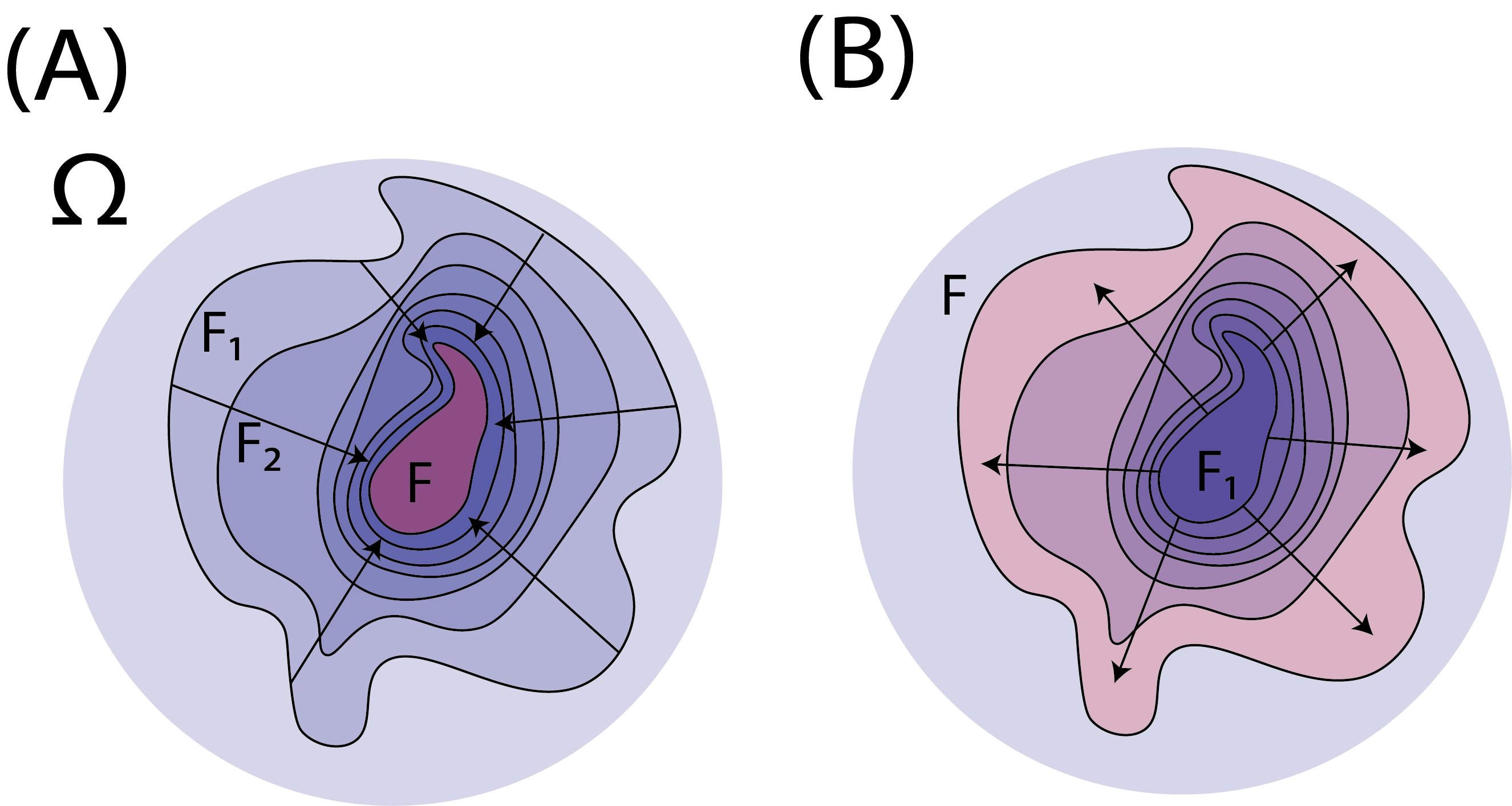
Fig. 2.5 Here we demonstrate convergence concepts for measures. (A) The sets \(F_n\) (in blue) converge to \(F\) (in red) from above. Notice that their measures get closer and closer to that of \(F\), from above, as well. (B) The sets \(F_n\) (in blue) converge to \(F\) (outermost set) from below. Notice that their measures get closer and closer to that of \(F\), from below, as well.#
Now, we’ll rattle off some other properties of measures. Try proving some of these as an exercise! Bonus: for your intuition, it is often extremely helpful to conceptualize these different properties with pictures like the above of your own.
Property 2.7 (Measure of difference)
Let \((\Omega, \mathcal F, \mu)\) be a measure space. If \(F_1, F_2 \in \mathcal F\) and \(F_1 \subseteq F_2\), then:
Property 2.8 (Measure of union)
Let \((\Omega, \mathcal F, \mu)\) be a measure space. If \(F_1, F_2 \in \mathcal F\), then:
Property 2.9 (Inclusion/Exclusion I)
Let \((\Omega, \mathcal F, \mu)\) be a measure space. If \(F_1, F_2 \in \mathcal F\) where \(\mu(F_1), \mu(F_2) < \infty\), then:
Property 2.10 (Inclusion/Exclusion II)
Let \((\Omega, \mathcal F, \mu)\) be a measure space. If \(n \in \mathbb N\) and \(\{F_m\}_{m \in [n]} \subseteq \mathcal F\) where for all \(m \in [n]\), \(\mu(F_m) < \infty\), then:
where \(F_\mathcal I \triangleq \cap_{m \in \mathcal M}F_m\).
2.2.2.2. Almost everywhere#
When making statements using measures, we might want to ascribe things to subsets of the sample space that might not, necessarily, hold true everywhere. As you will learn later in this book, in particular, we can say a lot of really useful things about the sample space that are, for all intents and purposes, nearly always true (but not, necessarily, absolutely always true). The key fine point here has to do with something called \(\mu\)-null elements of the \(\sigma\)-algebra:
Definition 2.32 (\(\mu\)-null element)
Let \((\Omega, \mathcal F, \mu)\) be a measure space. \(F \in \mathcal F\) is called \(\mu\)-null if \(\mu(F) = 0\).
Next, we’ll define the specific wording for what we are talking about here, which is called almost everywhere:
Definition 2.33 (Almost everywhere (a.e.))
Let \((\Omega, \mathcal F, \mu)\) be a measure space, and let \(\mathcal S : \Omega \rightarrow \{0, 1\}\) be a statement about points in the event space \(\Omega\) that is either true or false. The statement \(\mathcal S\) is said to hold almost everywhere (a.e.) if:
\(F = \{\omega \in \Omega : \mathcal S(\omega)\text{ is false}\} \in \mathcal F\), and
\(\mu(F) = 0\).
The first condition of this definition asserts that, for a statement to hold almost everywhere, the places it does not hold must all be an element of the \(\sigma\)-algebra \(\mathcal F\). Further, the places the statement does not hold true must be \(\mu\)-null. So, by almost everywhere, what we mean is that it holds everywhere that has an appreciable (non-zero) size (measure isn’t size persay, but it can be conceptualized that way). The first place we can put this into practice so you can get a feel for what we mean is in the construction of the Lebesgue measure, which is an invaluable tool we will use more in the later sections of this chapter.
2.2.2.3. Lebesgue measure#
So; why did we talk about \(\pi\)-systems at all in this book? It wasn’t just because we thought they were cool, or interesting, it is because they are essential tools for building out the Lebesgue measure, which we’ll learn about now.
The most interesting aspect of a \(\pi\)-system as it relates to probability theory is the following:
Lemma 2.4 (Uniqueness of extensions of measures from \(\pi\)-systems to \(\sigma\)-generated algebras)
Let \(\Omega\) be the event space, and suppose that \(\mathcal P\) is a \(\pi\)-system on \(\Omega\), where \(\mathcal F = \sigma(\mathcal P)\). Suppose that \(\mu_1, \mu_2\) are measures on the measurable space \((\Omega, \mathcal F)\). Further, suppose:
For every \(P \in \mathcal P\), \(\mu_1(P) = \mu_2(P)\), and
The measures are finite: \(\mu_1(\Omega) = \mu_2(\Omega) < \infty\).
Then for every \(F \in \mathcal F = \sigma(\mathcal P)\), \(\mu_1(F) = \mu_2(F)\).
To state this a little more succinctly, if two measures agree on a \(\pi\)-system, they also agree on the \(\sigma\)-algebra generated by that \(\pi\)-system. The “kind of” obscure second criterion, that the measures are finite, simply ensures that we don’t have a situation where we are trying to justify that \(\infty = \infty\), and in fact, this lemma turns out to be false if we omit this condition (while the reason it is false falls somewhat out of the scope of this book, we’d encourage you to look around and gain some intuition as to why).
Now is where the real magic happens:
Theorem 2.2 (Carothéodory’s Extension)
Let \(\Omega\) be an event space, let \(\mathcal A\) be an algebra on \(\Omega\), and let \(\mathcal F = \sigma(\mathcal A)\). Then if \(\mu_0 : \mathcal A \rightarrow \bar{\mathbb R}_{\geq 0}\) is a countably additive map, \(\exists \mu\) on \((\Omega, \mathcal F)\) s.t. \(\mu = \mu_0\) on \(\mathcal A\).
So, what is this telling us? This is telling us that, if we can define a measure on an algebra \(\mathcal A\), we can extend it to the \(\sigma\)-algebra generated by that algebra, \(\mathcal F = \sigma(\mathcal A)\), for free! Further, when we combine this with Lemma 2.4, we can also conclude that this measure is unique. Cool, right? Let’s see how this helps us for defining the Lebesgue measure:
Definition 2.34 (Lebesgue measure on \((\alpha, \beta]\))
Let \(\Omega = (\alpha, \beta]\), and define the algebra:
Then \(\mathcal A_\lambda\) is an algebra (and hence, also a \(\pi\)-system) on \(\Omega\), and \(\mathcal F_\lambda = \sigma(\mathcal A_\lambda) = \mathcal B(\alpha, \beta]\).
Let \(A \in \mathcal A_\lambda\). Define:
Then we define the Lebesgue measure \(\lambda\) to be the unique measure that extends \(\lambda_0\) from \(\mathcal A_\lambda\) to \(\mathcal F_\lambda\).
So, what is this statement saying? In effect, what we are doing here is first, we define an algebra that is pretty easy to understand: Basically, the sets in the algebra defined on \(\Omega\) are just all of the different ways that we could take (countable) unions of (non-overlapping) sub-intervals on \((\alpha, \beta]\). The \(\sigma\)-algebra generated by this algebra is, in fact, the Borel \(\sigma\)-algebra. We define a somewhat intuitive countably additive set function on this algebra, by just taking the value to be the sum of the (non-overlapping) interval lengths. Let’s see what elements of \(A_\lambda\) look like:

Fig. 2.6 An example of a set in \(\mathcal A_\lambda\), where \(k = 7\). \(\mathcal A_\lambda\) contains the set of the union of all of the points expressed by the intervals \((a_i, b_i]\), for \(k \in [7]\), shown above (the union of these items being a single set in \(\mathcal A_\lambda\)). It also includes all possible sets we could express in this way, where we could pick \(a_i\)s and \(b_i\)s, and still be left with \(\alpha \leq a_1 < b_1 \leq ... \leq a_7 < b_7 \leq \beta\). Finally, it repeats this for every single natural number, \(k \in \mathbb N\). On such a set, the measure \(\lambda_0\) is defined as the width of the intervals that the set is comprised of, shown in red.#
We don’t bother to describe the Lebesgue measure much more in-depth, because we don’t have to:
Theorem 2.3 (Existence and uniqueness of the Lebesgue measure)
Suppose the Lebesgue measure \(\lambda\) is defined as in Definition 2.34 on the measurable space \(\left(\Omega, \mathcal F_\lambda\right)\) where \(\Omega = (\alpha, \beta]\) is an interval. \(\lambda\) exists and is unique.
Proof. Existence: by Theorem 2.2, a measure \(\lambda^*\) as the measure that extends \(\lambda_0\) from \(\mathcal A_\lambda\) to \(\mathcal F_\lambda = \sigma(\mathcal A_\lambda)\) exists.
Uniqueness: By Lemma 2.4, since \(\mathcal A_\lambda\) is an algebra (and hence, also a \(\pi\)-system), this measure is unique on \(\mathcal F_\lambda = \sigma(\mathcal A_\lambda)\).
In effect, what this means is that the relatively intuitive description we gave in the definition for \(\lambda_0\) was plenty for us to know that there is a unique measure \(\lambda\) that behaves exactly this way on \(\mathcal A_\lambda\) (and extends it to \(\mathcal F_\lambda\)), and that measure is the Lebesgue measure.
If you’re careful, you’ll also notice that the measure we just defined has another interesting property: one of the sets in \(\mathcal A_\lambda\) is the set where \(k = 1\), and \(a_1 = \alpha\), and \(b_1 = \beta\). As you can see as we defined it, \(\lambda((a_1, b_1]) \equiv \lambda_0((a_1, b_1])= \beta - \alpha\). Further, note that \((a_1, b_1] = (\alpha, \beta] = \Omega\). This means that \(\lambda(\Omega) = \beta - \alpha\). Then if we were to take \(\beta = 1\) and \(\alpha = 0\), the Lebesgue measure in this case is something special: it is a probability measure. Let’s take a look at what this means.
2.2.3. Probability measures#
Finally, we are ready for the most important concept of this section: the probability measure. To define a probability measure, we really don’t need to do much: we just add a single property to the definition of measure. Since probability measures are measures (but reverse need not be true), all of those nice properties we just learned about measures extend to probability measures, too:
Definition 2.35 (Probability Measure)
Let \((\Omega, \mathcal F, \mu)\) be a measure space. We say that \(\mu\) is a probability measure if \(\mu(\Omega) = 1\), and we typically denote such measures with \(\mathbb P\).
Nothing to it: all we added was the condition that the measure, or the probability, of the entire event space was \(1\). Likewise, we have probability spaces:
Definition 2.36 (Probability Space)
The triple \((\Omega, \mathcal F, \mathbb P)\) is called a probability space, where:
\(\Omega\) is a set (the event space),
\(\mathcal F\) is a set of events, where \(\mathcal F\) is a \(\sigma\)-algebra on \(\Omega\),
\(\mathbb P: \mathcal F \rightarrow [0, 1]\) is a probability measure that assigns probabilities to events.
In that last definition, we snuck in a fact about probability measures \(\mathbb P\): that their upper bound is always \(1\) (e.g., \(\mathbb P\) ascribes values in \([0, 1]\)), which wasn’t quite what the definition of a probability measure states unless you look closely. This is a consequence of the fact that any \(F \in \mathcal F\) is a subset of \(\Omega\); e.g., \(F \subseteq \Omega\), so therefore \(\mathbb P(F) \leq \mathbb P(\Omega) = 1\), simply by Property 2.3.
2.2.3.1. Almost surely#
Now that we have probability measures under our belt, we are ready to adapt some lingo we used for measures to probability statements:
Definition 2.37 (Almost surely)
Let \((\Omega, \mathcal F, \mathbb P)\) be a probability space, and let \(\mathcal S : \Omega \rightarrow \{0, 1\}\) be a statement about points in the event space \(\Omega\) that are either true or false. The statement \(\mathcal S\) is said to hold almost surely (a.s.) if, with \(F = \{\omega \in \Omega : \mathcal S(\omega)\text{ is true}\} \in \mathcal F\), and \(\mathbb P(F) = 1\).
We can understand this to be, in effect, an (equivalent) reversal of what we said for almost everywhere in Definition 2.33. Whereas for almost everywhere, we asserted that the space on which the statement does not hold has measure \(0\), for almost surely, we asserted that the space on which the statement does hold has probability \(1\). But, if a statement holds almost surely, it holds almost everywhere, as with \(F\) as above, then \(F^c = \Omega \setminus F = \{\omega \in \Omega : \mathcal S(\omega)\text{ is false}\}\):
the language “almost surely” is typically just used to make explicit the fact that the measure that the statement holds with respect to is a probability measure.