2.4. Pushforward measures and distribution functions#
So, now we have these concepts called random variables, which are really just measurable functions on a particular domain with respect to some codomain. We can perform all of the traditional mathematical operations with random variables, and still obtain random variables. What else do we need as far as machinery goes? We need to link these random variables to probabilities. This happens via a concept called a pushforward measure.
2.4.1. Pushforward measure#
As it turns out, we can use measurable functions defined on a measure space to obtain measures on the codomain. This process is called “pushing forward” the measure from one measure space to the measurable space in the codomain, via the measurable function:
Definition 2.40 (Pushforward measure)
Suppose that \((\Omega, \mathcal F, \mu)\) is a measure space, and \((S, \Sigma)\) is a measurable space, where \(X \in m(\mathcal F, \Sigma)\). Then the pushforward of \(\mu\) is defined as the measure \(X_*\mu : \Sigma \rightarrow \bar{\mathbb R}_{\geq 0}\) where for every \(B \in \Sigma\):
The idea here is that we are, in some sense, finding which values of \(\Omega\) were mapped into \(B\) by \(X\) via \(X^{-1}(B)\) (which must be a set \(F \in \mathcal F\), by definition of a random variable), and then calculating the measure (via \(\mu\)) of this set. Since \(\mu\) is a measure with respect to the measurable space \((\Omega, \mathcal F)\), this is a possible thing that we can do.
Let’s consider this from another angle to describe what’s going on here. First, we know that \(X : \Omega \rightarrow S\); that is, \(X\) is mapping elements of the event space to the codomain. \(X^{-1} : \Sigma \rightarrow \mathcal F\) (the definition of a \((\mathcal F, \Sigma)\)-random variable) takes us from subsets of the codomain (elements of \(\Sigma\)) to measurable subsets of the sample space (elements of \(\mathcal F\)). We can then use \(\mu\) to measure these measurable subsets of the sample space.
Conceptually, we can understand this process using the the intuition we gained from random variables, and combine it with what we learned about measures:
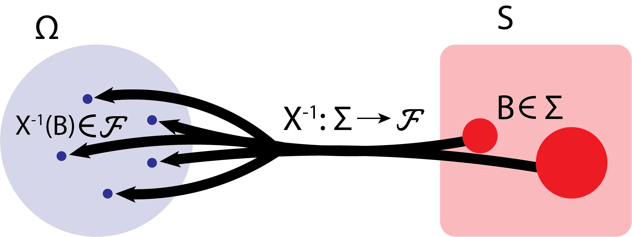
Fig. 2.9 We start with some subset of \(S\), \(B\) (in red), which is in the \(\sigma\)-algebra defined on the codomain, \(\Sigma\). We identify the corresponding element of the domain (here, denoted \(X^{-1}(B)\), in blue) that is mapped somewhere within \(B\), which is an element of the \(\sigma\)-algebra defined on the domain, \(\mathcal F\) (since \(X\) is \((\mathcal F, \mathcal \Sigma)\) measurable). To compute the pushforward of \(X\) with respect to the set \(B\), we simply evaluate the measure (the area, which is defined on the measurable space \((\Omega, \mathcal F)\)) of these corresponding blue circles. This is denoted by \(X_*\mu(B)\), giving us a measure of the codomain.#
It is called a pushforward because we are “pushing” the measure from one measurable space to the other. We will learn more about the pushforward measure when we try to compute measure-theoretic integrals, but for now all that we need to know is that it’s a measure. To do this, we’ll need a quick lemma:
Lemma 2.6 (Preimage of disjoint sets are disjoint)
Suppose that \((\Omega, \mathcal F, \mu)\) is a measure space, and \((S, \Sigma)\) is a measurable space, where \(X \in m(\mathcal F, \Sigma)\). Let \(\{F_n\}_{n \in \mathbb N} \subseteq \mathcal F\) that are disjoint. Then \(\{X^{-1}(F_n)\}_{n \in \mathbb N}\) where \(X^{-1}(F_n) \equiv \{X \in F_n\} \equiv \{\omega \in \Omega : X(\omega) \in F_n\}\) are disjoint.
Proof. It suffices to show that if \(\omega \in X^{-1}(F_n)\), then for all \(m \neq n\), \(\omega \not \in X^{-1}(F_m)\), by definition of disjointness.
Suppose that \(\omega \in X^{-1}(F_n) \equiv \{\omega \in \Omega : X(\omega) \in F_n\}\), so \(X^{-1}(\omega) \in F_n\).
Since \(F_n\) are disjoint, and \(X\) is a function (no \(\omega \in \Omega\) can be mapped to multiple values in the codomain), then for all \(m \neq n\), \(\omega \not \in X^{-1}(F_m)\).
And now we are ready to prove the result we intended to:
Lemma 2.7 (Pushforward measure is a measure)
Suppose that \((\Omega, \mathcal F, \mu)\) is a measure space, and \((S, \Sigma)\) is a measurable space, where \(X \in m(\mathcal F, \Sigma)\), and let \(X_*\mu : \Sigma \rightarrow \bar{\mathbb R}_{\geq 0}\) be the pushforward measure of \(\mu\). Then \(X_*\mu\) is a measure.
Proof. To show that \(X_*\mu\) is a measure, we need to show that it is non-negative, countably additive, and that the measure of the empty set is \(0\).
1. Non-negative: Suppose that \(B \in \Sigma\).
Since \(X \in m(\mathcal F, \Sigma)\), then \(X^{-1}(B) \in \mathcal F\).
Then since \(\mu\) is a measure on \((\Omega, \mathcal F)\), \(\mu(X^{-1}(B)) \equiv X_*\mu(B) \geq 0\) (\(X_*\mu\) retains non-negativity).
2. Countably additive: Suppose that \(\{B_n\}_{n \in \mathbb N} \Sigma\) are disjoint. Then:
which follows by Lemma 2.6, since the preimage of disjoint sets are disjoint. Continuing, and noting that \(\mu\) is a measure means that it is countably additive:
as desired. 3. Measure of empty set is \(0\): Notice that \(X^{-1}(\varnothing) = \varnothing\).
Then since \(\mu\) is a measure:
2.4.2. Inducing distribution functions#
Now that we have random variables (measurable functions), if the domain is a probability space, we can use the definition of a random variable to deduce that it is certainly the case that for any set in the codomain, the preimage of the set in the codomain is in the \(\sigma\)-algebra of the corresponding probability space. Since this set is in the \(\sigma\)-algebra of the probability space, we can assign a probability to that set:
Definition 2.41 (Law of a random variable)
Suppose the probability space \((\Omega, \mathcal F, \mathbb P)\) and the measurable space \((S, \Sigma)\), where \(X \in m(\mathcal F, \Sigma)\) is a random variable. Then the induced probability measure on \(S\) by \(X\), also known as the law of \(X\), is the measure \(\mathcal L_X\) where for every \(B \in \Sigma\):
We call this particular induced probability measure the law of \(X\) because, as we will see shortly, it ascribes most of the behaviors about \(X\) that we will care about. In other words, using compositions, we could describe \(\mathcal L_X \triangleq \mathbb P \circ X^{-1}\). \(\mathcal L_X\) represents the probability (the measure of the domain \(\Omega\)) that under \(X\), winds up in \(B\).
Based on what we just learned about pushforward measures, it’s pretty clear that the law is a measure (since probability measures are measures), so \(\mathcal L_X \equiv X_*\mathbb P\), using the notation we became familiar with for pushforward meassures. This means that the intuition that we just covered about pushforward measures extends directly to the law, too.
We really only need one new attribute from the preceding proof to show that the law is a probability measure:
Proposition 2.1 (The law is a probability measure)
Suppose the probability space \((\Omega, \mathcal F, \mathbb P)\) and the measurable space \((S, \Sigma)\), where \(X \in m(\mathcal F, \Sigma)\) is a random variable, and \(\mathcal L_X = \mathbb P\circ X^{-1}\) is the law of \(X\). \(\mathcal L_X\) is a probability measure on \((S, \Sigma)\).
Proof. 1. \(\mathcal L_X(S) = 1\):
which follows because \(X : \omega \mapsto X(\omega) \in S\) for any \(\omega\) by definition of \(X : \Omega \rightarrow S\).
The non-negativity and countable additivity conditions for the law \(\mathcal L_X\) are proven by Lemma 2.7.
If the codomain is the measurable space \((\mathbb R, \mathcal R)\), we are ready to make a further claim about \(\mathcal L_X\) using the distribution function:
Definition 2.42 (Distribution function)
Suppose that \((\Omega, \mathcal F, \mathbb P)\) is a probability space, and the measurable space \((\mathbb R, \mathcal R)\), where \(X \in m(\mathcal F, \mathcal R)\) is a random variable with law \(\mathcal L_X\). The distribution function is:
As it turns out, the distribution function fully determines the law:
Theorem 2.6 (The distribution function fully determines the law of a random variable)
Suppose that \((\Omega, \mathcal F, \mathbb P)\) is a probability space, and the measurable space \((\mathbb R, \mathcal R)\), where \(X \in m(\mathcal F, \mathcal R)\) is a random variable. Then \(\mathcal L_X\) is fully determined by the function \(F_X : \mathbb R \rightarrow [0, 1]\).
Proof. Note that \(\mathcal P = \left\{(-\infty, r] : r \in \mathbb R\right\}\) is a \(\pi\)-system on \(\mathbb R\), where \(\sigma(\mathcal P) = \mathcal R\).
Further, note that on \(\mathcal P\), that for any \(r \in \mathbb R\), \(\mathcal L((-\infty, r]) = F_X(r)\), by definition, so \(\mathcal L_X\) and \(F_X\) agree on all of \(\mathcal P\).
Then by Lemma 2.4, \(\mathcal L_X = F_X\) on \(\sigma(\mathcal P) = \mathcal R\).
In general, when we work with random variables, we will work with the distribution function for many of our proofs that we consider.
Remark 2.7 (The codomain will be \((\mathbb R, \mathcal R)\))
For the remainder of this section, we will work where the codomain is the measurable space \((\mathbb R, \mathcal R)\). For this reason, we’ll omit explicitly stating the codomain every single time for brevity.
Let’s break down how distribution functions work:

Fig. 2.10 (A) \(X\) is a \(\mathcal F\) random variable on the measure space \((\Omega, \mathcal F)\) which assigns points in \(\Omega\) to values on \(\mathbb R\). As \(r_i\) increases, large and larger subsets of points (indicated by the sequentially increasing sets, going from red, to blue, to green) in \(\Omega\) take a value \(X(\omega)\) that is less than \(r_i\). (B) The distribution function corresponds to the relative size of the sets (the probability) in \(\Omega\) for points which land in different intervals of \(\mathbb R\).#
2.4.3. Properties of distribution functions#
Distribution functions have some nice properties that will be convenient for building up intuition about the law of random variables. First up is monotonicity:
Property 2.19 (Monotonicity of distribution functions)
Suppose the probability space \((\Omega, \mathcal F, \mathbb P)\), and that \(X \in m\mathcal F\) is a random variable with distribution function \(F\). Then if \(x \leq y \in \mathbb R\), \(F(x) \leq F(y)\).
Proof. Since \(x \leq y\), then:
Then since \(\mathbb P\) is a measure, Property 2.3, \(F(x) \equiv \mathbb P(X \leq x) \leq \mathbb P(X \leq y) \equiv F(y)\).
So, what this establishes is that \(F\) is monotone non-decreasing. Further, we can establish properties about the tails of \(F\), too. These results borrow the monotone convergence (from above and below) of measures:
Property 2.20 (Tails of the distribution function)
Suppose the probability space \((\Omega, \mathcal F, \mathbb P)\), and that \(X \in m\mathcal F\) is a random variable with distribution function \(F\). Then \(\lim_{x \rightarrow \infty}F(x) = 1\), and \(\lim_{x \rightarrow -\infty}F(x) = 0\).
Proof. 1. Suppose that for \(n \in \mathbb N\), \(x_n \uparrow \infty\).
Then with \(A_n = \{X \leq x_n\} \equiv \{\omega : X(\omega) \leq x\}\), it is clear that \(A_n \uparrow \Omega\) as \(n \rightarrow \infty\). This follows because the codomain for \(X\), \((\mathbb R, \mathcal R)\), is upper-bounded by \(\infty\).
Then:
where the convergence from below is by Property 2.5.
2. Suppose that for \(n \in \mathbb N\), \(x_n \downarrow -\infty\).
Then with \(A_n = \{X \leq x_n\}\), it is clear that \(A_n \downarrow \varnothing\) as \(n \rightarrow \infty\). This is because the codomain for \(X\) is lower-bounded by \(-\infty\).
Then:
where the convergence from above is by Property 2.6.
Another property we will make substantial use of with respect to distribution functions is that they are right continuous, and not (necessarily) left-continuous:
Property 2.21 (Right-continuity of distribution function)
Suppose the probability space \((\Omega, \mathcal F, \mathbb P)\), and that \(X \in m\mathcal F\) is a random variable with distribution function \(F\). \(\lim_{y \downarrow x}F(y) = F(x)\).
Proof. Suppose that \((x_n)_{n \in \mathbb N} \subset \mathbb R\) is a countable sequence where \(x_n \downarrow x\), and \(x \not \in (x_n)_{n \in \mathbb N}\). Such a sequence exists, by the completeness of the reals.
Note that for any such \(x_n\), that \(A_n \triangleq \{\omega : X(\omega) \leq x_n\} \supset \{\omega : X(\omega) \leq x\}\), since \(x_n > x\).
Further, note that \(\bigcap_{n \in \mathbb n} A_n = \{X \leq x\} \equiv \{\omega : X(\omega) \leq x\}\), because for any \(\epsilon\), \(\exists N\) s.t. for all \(m > N\), \(x_m - x < \epsilon\), by definition of \(x_n \downarrow x\) as \(n \rightarrow \infty\).
Then:
where the convergence from above is by Property 2.6.
The key fine point here for the (potential) lack of left-continuity is that, as we see here, the right-hand side of the following equality is \(\mathbb P(X < x)\), and not \(F(x) = \mathbb P(X \leq x)\):
Property 2.22 (Distribution functions (not necessarily) left-continuous)
Suppose the probability space \((\Omega, \mathcal F, \mathbb P)\), and that \(X \in m\mathcal F\) is a random variable with distribution function \(F\). Then \(F(x^-) \triangleq \lim_{y \uparrow x}F(y) = \mathbb P(X < x)\).
Proof. Suppose that \((x_n)_{n \in \mathbb N}\subset \mathbb R\) is a countable sequence where \(x_n \uparrow x\), and \(x \not \in (x_n)_{n \in \mathbb N}\). Such a sequence exists, by the completeness of the reals.
Note that for any such \(x_n\), that \(A_n \triangleq \{X \leq x_n\} \equiv \{\omega : X(\omega) \leq x_n\} \subset \{\omega : X(\omega) \leq x\} \equiv \{X \leq x\}\), since \(x_n > x\).
Further, note that \(\bigcup_{n \in \mathbb N}A_n = \{\omega : X(\omega) < x\}\). This follows because \(x \not \in (x_n)_{n \in \mathbb N}\) by construction, and by applying the definition of the countable set union. This holds for any countable sequence as-described.
Then:
where the convergence from below is by Property 2.5.
Finally, the probability at any particular point can be taken to be the difference in the distribution function at that value, minus the limit point we defined above:
Property 2.23 (Probability at a point)
Suppose the probability space \((\Omega, \mathcal F, \mathbb P)\), and that \(X \in m\mathcal F\) is a random variable with distribution function \(F\). Then \(\mathbb P(X = x) = F(x) - F(x^-)\).
Proof. Note that \(\{\omega : X(\omega) = x\} = \{\omega : X(\omega) \leq x\} \setminus \{\omega : X(\omega) < x\}\).
Further, note that \(\{\omega : X(\omega) \leq x\} \supseteq \{\omega : X(\omega) < x\}\). Then by Property 2.7, since \(\mathbb P\) is a measure: