3.2. Properties of Integration#

That last section was pretty neat stuff, eh?

While this might seem like all we did was introduced a bunch of cumbersome notation to “reinvent the wheel” and give you back your Riemann integral from calculus, it turns out this is a lot more powerful than that stuff. In particular, you’ll notice that we were extremely cautious every step of the way from the preceding chapters all the way to now regarding which assumptions different conditions hold under. These might seem like “mindless details” that you’d rather go without, but the brilliance of probability theory is the details.

These properties that we are constructing, from the ground up, have been explicit about every assumption made along the way. As we build more and more results, we’re going to keep that trend up, and all these assumptions and conditions are going to start making sense as you begin to see that extremely weak conditions might add up to a result that is beautiful. As you’ll see in the next section, the concept of expected value in probability theory is understood as a special case of integration with respect to a probability measure, so while we’re going to unfortunately burden you with some more properties of integrals, it will start to tie back to probability theory more directly next.

3.2.1. Norms and Convexity#

In this section, we’ll learn some details about two concepts that we will later see are acutely related: norms and convex functions. When we attempt to classify random variables in the next chapter, we’ll use these two concepts to do so.

3.2.1.1. Convex Functions#

We’ll start off with a definition you’ve probably seen in some form before:

Definition 3.11 (Convex Function)

A function $\varphi : \mathcal X \rightarrow \mathbb R$ defined on a convex subset $\mathcal X \subseteq \mathbb R$ is convex if for all $\lambda \in (0, 1)$ and for all $x_1, x_2 \in \mathcal X$:

\[ \lambda\varphi(x_1) + (1 - \lambda)\varphi(x_2) \geq \varphi\left(\lambda x_1 + (1 - \lambda)x_2\right).\]

Let’s think about what this means, intuitively. First: what the heck is a convex subset $\mathcal X$? All that this means is, for all $x_1, x_2 \in \mathcal X$, that any possible convex combination of these elements $\lambda x_1 + (1 - \lambda)x_2$ is also $\in \mathcal X$. This holds for all $\lambda \in (0, 1)$. For instance, if we are dealing with real numbers, $\mathcal X$ could just be an interval.

The idea here is that in this case, the point $z = \lambda x_1 + (1 - \lambda)x_2$ is some point in between $x_1$ and $x_2$. This is ensured by the fact that $\lambda$ is between $0$ and $1$. Now, let’s think about the left side of an equation. What happens as $t$ changes? Graphically, it turns out that it looks something like this:

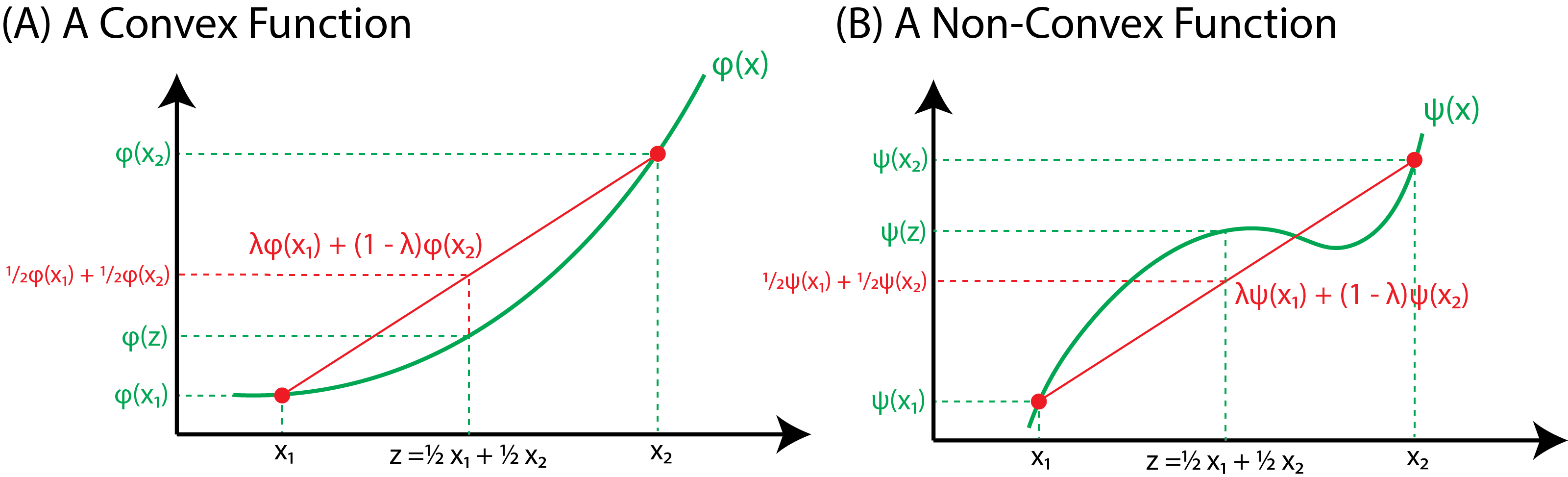
../../_images/convex.png — Fig. 3.2 **(A)** The red line represents the line $\lambda \varphi(x_1) + (1 - \lambda)\varphi(x_2)$ for some value $\lambda \in (0, 1)$. For a convex function, for any two points $x_1$ and $x_2$, this line will be *entirely* above the actual function, $\varphi(x)$. **(B)** A non-convex function $\psi$. Notice that we can choose points $x_1$ and $x_2$ where the red line is not always above the function.#

An important consequence that we will use throughout this course is a relatively simple real analysis result:

Lemma 3.5 (Convex functions and second derivatives)

A function $\varphi \in C^2 : \mathcal X \rightarrow \mathbb R$ defined on an interval $\mathcal X$ is convex on $\mathcal X$ if and only if for all $x \in \mathcal X$, $\varphi''(x) \geq 0$.

What this asserts is that if the function $\varphi$ is further twice differentiable and the function is defined on an interval (which is a convex subset), we have a second way to assert convexity, which is (often) much easier to work with: simply check its second derivative. Visually, this solidifies an intuitive notion of convexity demonstrated by Fig. 3.2(A): a convex function will be curved upwards.

Now, we’re going to talk about some nuancy points that are consequences of the definition of convex functions. In my opinion, the proofs/intuition of these results go somewhat beyond an introductory real analysis course, so you shouldn’t worry if it doesn’t immediately make sense to you:

Lemma 3.6 (Subderivatives of convex functions)

Suppose that the function $\varphi : \mathcal X \rightarrow \mathbb R$ defined on a convex open subset $\mathcal X \subseteq \mathbb R$ is convex. The the subderivative at a point $x_0 \in \mathcal X$ is a real number $c$ s.t. for all $x \in \mathcal X$:

\[ c \leq \frac{\varphi(x) - \varphi(x_0)}{x - x_0}.\]

That $\mathcal X$ is open suggests that if $x \in \mathcal X$, that the neighborhood $\{x + h\}_{0 < h < \epsilon} \subseteq \mathcal X$ for some $\epsilon > 0$. As it turns out, for a convex function $\varphi$, we can take this even further, and can say that:

\[\begin{split} a_l &= \lim_{h \downarrow 0}\frac{\varphi(x) - \varphi(x - h)}{h} \\ a_u &= \lim_{h \downarrow 0}\frac{\varphi(x + h) - \varphi(x)}{h}\end{split}\]

are both finite, and $[a_l, a_u]$ is called the subdifferential (it is a set of all of the subdifferentials). When the function $f$ is continuously differentiable on the entire domain $\mathcal X$, this is fairly rudimentary what we are talking about here: $a_l$ and $a_u$ are the left and right derivatives for a point $x$ (and, in the case of continuous functions, these are equal). The nuance here can be shown with something that is convex but not continuously differentiable, like the absolute value:

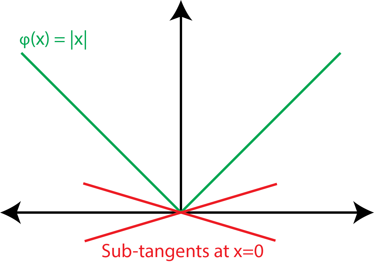
../../_images/subderiv.png — Fig. 3.3 In this case, we can see two sub-tangent lines at the point $x = 0$, which are lines which intersect with $f(x) = |x|$ at $x = 0$ but whose slopes are in the interval formed by the left and right derivatives, $-1$ and $1$ respectively. The sub-derivatives exist since $f(x) = |x|$ is convex; if you are struggling with why it is convex, think about the lines we drew previously in Fig. 3.2.#

Now we get to one of the fundamental results of integration:

Theorem 3.2 (Jensen’s Inequality)

Suppose that:

$(\Omega, \mathcal F, \mathbb P)$ is a probability space,
$\mathcal X \subseteq \mathbb R$ is an interval,
$f \in m\mathcal F : \Omega \rightarrow \mathcal X$ is a measurable function,
$\varphi \in m\mathcal R: \mathcal X \rightarrow \mathbb R$ is convex, and
$f$ and $\varphi(f) = \varphi \circ f$ are $\mathbb P$-integrable.

Then:

\[ \varphi\left(\int f \,\text d \mathbb P\right) \leq \int \varphi\left(f\right) \,\text d \mathbb P.\]

This result, it turns out, is pretty easy to prove if $f$ is also $C^2$, but that wouldn’t quite be as general as we want it to be: this result can hold for any convex functions, not just the $C^2$ ones. In the proof below, we use the concept of the sub-derivative that we just intuited our way through, and then we’ll recap why we had to use sub-derivatives at all once we’re done:

Proof. Let $c = \int f \,\text d\mathbb P$, which is finite since $f$ is $\mathbb P$-integrable Definition 3.10.

Let $\ell(x) = a x + b$ be a linear function for $a, b, x \in \mathbb R$ s.t. $\ell(c) = \varphi(c)$, and $\varphi(x) \geq \ell(x)$. Such a function $\ell$ exists, since by the convexity of $\varphi$, we can see that with:

\[ a_l = \lim_{h \downarrow 0}\frac{\varphi(c) - \varphi(c - h)}{h} \leq \lim_{h \downarrow 0}\frac{\varphi(c + h) - \varphi(c)}{h} = a_u,\]

Letting $a \in [a_l, a_u]$ ($a$ is a sub-derivative of $\varphi$) and $\ell(x) = a(x - c) + \varphi(c)$ gives the desired properties, as:

\[\begin{split} x \neq c \Rightarrow \ell(x) &\leq a_u(x - c) + \varphi(c),\,\,\,\,\text{defn. of a sub-derivative}, a \leq a_u \\ x = c \Rightarrow \ell(c) &= \varphi(c).\end{split}\]

Note, then, that $\varphi(x) \geq \ell(x)$ for any $x \in \mathbb R$, and consequently, $\varphi \circ f \geq \ell \circ f$, so $\varphi \circ f \overset{a.e.}{\geq} \ell \circ f$.

It is pretty that $\ell \circ f$ is a rescaling of an integrable function $f$ by $a$ and a sum with a constant term, $-ac + \varphi(c)$. Particularly, here note that since we have a probability space, the measure of the entire space is finite, and the constant is integrable by Remark 3.1. Therefore, $\ell \circ f$ is integrable by Property 3.11 and Property 3.12.

Then by Corollary 3.1, since $\varphi \circ f$ is integrable by supposition:

\[\begin{split} \int \varphi\circ f \, \text d\mathbb P &\geq \int \ell \circ f \, \text d\mathbb P \\ &= \int \left(a f - c + \varphi(c)\right) \, \text d\mathbb P \\ &= a\left(\int f\,\text d \mathbb P - c\right) + \varphi(c) \\ &= \ell\left(\int f\,\text d\mathbb P\right),\,\,\,\,\ell(x) \triangleq a(x - c) + \varphi(c) \\ &= \varphi\left(\int f \, \text d \mathbb P\right),\,\,\,\,\ell(c) = \varphi(c)\end{split}\]

where by construction, $c = \int f \,\text d \mathbb P$.

So: why did we have to use sub-derivatives, and what did they let us do? Well, since $\varphi$ is only convex, it is entirely possible that the derivative doesn’t exist at a point we are interested in (think about if the absolute value had an inflection right at $x = \int f \,\text d \mathbb P$ instead of at $x = 0$, like in the figure we considered; e.g., $\varphi(x) = \left|x - \int f \,\text d \mathbb P\right|$). So, what we did was, we constructed a sub-tangent line via a sub-derivative at this point, just to give us extra protection for the general case where we could have a non-existant derivative.

3.2.1.2. Norms#

Jensen’s inequality will make properties about norms of random variables very easy to prove. What’s a norm you might ask?

Definition 3.12 (Functional norm)

Suppose that $(\Omega, \mathcal F, \mu)$ is a measure space, and suppose that $p \in [1, \infty)$. The functional norm of a function $f \in m\mathcal F : \Omega \rightarrow \mathbb R$ is:

\[||f||_p \triangleq \left(\int |f|^p \,\text d \mu\right)^{\frac{1}{p}}\]

We tend to classify functions as those that have finite functional norms:

Definition 3.13 ($\mathbb L^p$ space)

Suppose that $(\Omega, \mathcal F, \mu)$ is a measure space, and suppose that $p \in [1, \infty)$. Then the $\mathbb L^p(\mu)$ space is the set of measurable functions:

\[ \mathbb L^p(\mu) \triangleq \left\{f \in m\mathcal F : ||f||_p < \infty\right\}\]

We can use functional norms to obtain some more desirable properties of integration. Let’s check out Hölder’s inequality:

Theorem 3.3 (Hölder’s inequality)

Suppose that $(\Omega, \mathcal F, \mu)$ is a measure space, that $f, g \in m\mathcal F$, and that $p, q \in [1, \infty)$ are s.t. $\frac{1}{p} + \frac{1}{q} = 1$. Then:

\[ \int |f \cdot g| \,\text d \mu \leq ||f||_p ||g||_q.\]

Proof. If $||f||_p = 0$, then note that by definition, $\mu\left(\{\omega : f(\omega) \neq 0\}\right) = 0$ and so $f \overset{a.e.}{=} 0$, and vice-versa for $||g||_q$.

In this case, the product $f \circ g \overset{a.e.}{=} 0$, as $(f\cdot g)(\omega) \equiv f(\omega)g(\omega) = 0$ as well, satisfying the inequality.

Therefore, suppose that $||f||_p, ||g||_q > 0$. Further, WOLOG, assume that $||f||_p = ||g||_q = 1$. Note that this applies generally, as we could simply take $f'(\omega) = \frac{f(\omega)}{||f||_p}$ and vice-versa for $g$, and we would obtain a result that is simply a scalar multiple of $||f||_p||g||_q$, since $|f(\omega) g(\omega)| = ||f||_p||g||_q|f'(\omega)g'(\omega)|$ since by definition, $||f||_p, ||g||_q > 0$.

Note that for any $x, y \geq 0$, that using basic properties of the $\exp$ and $\log$ functions:

\[\begin{split} xy &= \exp(\log(xy)) \\ &= \exp(\log x + \log y) \\ &= \exp\left(\frac{1}{p} p\log x + \frac{1}{q}q \log y\right) \\ &= \exp\left(\frac{1}{p} \log x^p + \frac{1}{q} \log y^q\right)\end{split}\]

Notice that $\exp(x)$ is convex, since its second derivative is positive by Lemma 3.5. Then since $\frac{1}{p} + \frac{1}{q}$ is positive:

\[\begin{split} xy &\leq \frac{1}{p} \exp(\log x^p) + \frac{1}{q} \exp(\log y^q) \\ &= \frac{x^p}{p} + \frac{y^q}{q}.\end{split}\]

Taking $x = |f(\omega)|$ and $y = |g(\omega)|$, we see that:

\[ |f(\omega)||g(\omega)| = |f(\omega)g(\omega)| \leq \frac{|f(\omega)|^p}{p} + \frac{|g(\omega)|^q}{q},\]

which holds for all $\omega \in \Omega$, so $|f \cdot g| \leq \frac{|f|^p}{p} + \frac{|g|^q}{q}$. Integrating:

\[\begin{split} \int |f \cdot g| \,\text d \mu &\leq \int \left(\frac{|f|^p}{p} + \frac{|g|^q}{q}\right)\,\text d \mu \\ &= \frac{||f||_p}{p} + \frac{||g||_q}{q} \\ &= \frac{1}{p} + \frac{1}{q},\,\,\,\,||f||_p = ||g||_q = 1\text{ WOLOG} \\ &= 1,\,\,\,\,\frac{1}{p} + \frac{1}{q} \text{ by supposition} \\ &= ||f||_p ||g||_q.\end{split}\]

3.2.2. Convergence Results#

3.2.2.1. Convergence Concepts#

Next, we get to the convergence theorems for integrals. To do this, we first need two quick definitions to get us started:

Definition 3.14 (Convergence Almost Everywhere)

Suppose the measure space $(\Omega, \mathcal F, \mu)$, and the measurable functions $f, f_n \in m\mathcal F$, for all $n \in \mathbb N$. We say that $f_n \xrightarrow[n \rightarrow \infty]{a.e.} f$ if:

\[ \mu\left(\left\{\omega \in \Omega : \lim_{n \rightarrow \infty}f_n(\omega) \neq f(\omega)\right\}\right) \equiv \mu(\lim_{n \rightarrow \infty}f_n \neq f) = 0.\]

The idea here is that for all but a set of measure $0$, $f_n(\omega) \xrightarrow[n \rightarrow \infty]{} f(\omega)$. Stated another way, we have pointwise convergence of $f_n$ to $f$ almost everywhere.

We can also understand this definition using the concept of the $\limsup$ of a set, in an $\epsilon$ sort of way like you are used to in real analysis:

Definition 3.15 (Equivalent definition for convergence almost everywhere)

\[ \mu\left(\limsup_{n \rightarrow \infty}\left\{\omega \in \Omega : |X_n(\omega) - X(\omega)| > \epsilon\right\}\right) = 0.\]

In this definition, the intuition is that we are focusing on a sequence of sets (indexed by $n$) which are the points $\omega$ of the sample space $\Omega$ which are not $\epsilon$-close to $f(\omega)$. These are the sets of the form:

\[ \left\{\omega \in \Omega : |f_n(\omega) - f(\omega)| > \epsilon\right\}_{n \in \mathbb N}.\]

Remember that $\limsup_{n \rightarrow \infty}$ of a sequence of sets can be more specifically be understood to be the $\inf_{n \rightarrow\infty}\sup_{m \geq n}$, so we are concerned with the $\inf$ of sets of the form:

\[ F_n = \sup_{m \geq n}\left\{\omega \in \Omega : |X_m(\omega) - X(\omega)| > \epsilon\right\}\]

So, the interpretation of $F_n$ here is that it’s the largest possible measurable set of the sample space where for every $m \geq n$, $|f_m(\omega) - f(\omega)| > \epsilon$ (which is the definition of $f_m(\omega)$ not being $\epsilon$-close to $f(\omega)$ which is a condition for the limit to be $f(\omega)$). The nuance here is that we use a supremum, which is because it’s not immediately clear that the largest possible set that fulfills this criterion will necessarily be measurable (but, as-per Property 2.17, we know for sure that the supremum is measurable).

By construction, since $n$ is increasing, notice that $\{F_n\}_{n \in \mathbb N}$ are monotone non-increasing: $F_n \supseteq F_{n + 1}$, for all $n \in \mathbb N$. Intuitively, since it is bounded (from below by $\varnothing$) and monotone non-increasing, the infimum of these sequences of sets exist (by Lemma 2.3). We know for sure that the resulting set is further measurable by just checking Property 2.16.

Next, we get to a practically distinct definition, which almost looks the same. This concept is called convergence in measure:

Definition 3.16 (Convergence in measure)

\[ \mu\left(\left\{\omega \in \Omega : |f_n(\omega) - f(\omega)| > \epsilon\right\}\right) \equiv \mu(|f_n - f| > \epsilon) \xrightarrow[n \rightarrow \infty]{} 0.\]

While these definitions almost look the same, the practical distinction is that the limit, this time, is outside of the measure statement. The idea here is that, as $n$ grows, the measure of the set of points $\omega$ where $f_n(\omega)$ is not $\epsilon$-close to $f(\omega)$ is converging to zero. This contrasts from the fact that in the preceding statement, the measure of the set of points $\omega$ where $f_n(\omega)$ is not $\epsilon$-close to $f(\omega)$ as $n \rightarrow \infty$ is zero. Intuitively, convergence almost everywhere, in fact, implies convergence in measure (with the slight note that the entire space $\Omega$ must have finite measure). Let’s formalize this up a bit:

Lemma 3.7 (Convergence almost everywhere implies convergence in measure)

Suppose the measure space $(\Omega, \mathcal F, \mu)$, and the measurable functions $f, f_n \in m\mathcal F$, for all $n \in \mathbb N$, where $\{f_n\}_{n \in \mathbb N} \subset m\mathcal F$. If $f_n \xrightarrow[n \rightarrow \infty]{a.e.} f$ and $\mu(\omega) < \infty$, then $f_n \xrightarrow[n \rightarrow \infty]{} f$ in measure.

Proof. Suppose that $f_n \xrightarrow[n \rightarrow \infty]{a.e.} f$.

Let $\Omega_1 \triangleq \{\omega \in \Omega : \lim_{n \rightarrow \infty}f_n(\omega) = f(\omega)\}$, and $\Omega_1^c = \Omega \setminus \Omega_1$. By construction, note that $\mu(\Omega_1^c) = 0$.

By definition of $\xrightarrow[n \rightarrow \infty]{a.e.}$, then $\mu(\Omega_1^c) = 0$. Fix $\epsilon > 0$, and consider the sequence of sets:

\[F_n \triangleq \bigcup_{m \geq n}\left\{|f_n - f| > \epsilon\right\}.\]

By construction, note that $F_n \supseteq F_{n + 1}$, where $F_n \downarrow F_\infty = \bigcap_{n \in \mathbb N}F_n$.

Further, note that by design, for any $\omega \in \Omega_1$, that $\lim_{n \rightarrow \infty}f_n(\omega) = f(\omega)$. Then for any $\epsilon > 0$, there exists $N_\epsilon$ s.t. for all $n \geq N_\epsilon$, $|f_n(\omega) - f(\omega)| \leq \epsilon$, by definition of a limit.

Then for all $n > N_\epsilon$, $\omega \not \in F_n$, and consequently $\omega \not \in F_\infty$.

Then $F_\infty \cap \Omega_1 = \varnothing$; that is, $F_\infty \subseteq \Omega_1^c$.

Then by definition of a measure, $\mu(F_\infty) \leq \mu(\Omega_1^c) = 0$ by the way we constructed $\mu(\Omega_1)^c$. Further, since measures are lower-bounded by $0$, this implies that $\mu(F_\infty) = 0$.

Then since $F_n \downarrow F_\infty$:

\[\begin{split} \mu(|X_n - X| > \epsilon) &\leq \mu(F_n),\,\,\,\,\{|X_n - X| > \epsilon\} \subseteq F_n \\ &\downarrow \mathbb P(A_\infty) = 0\text{ as $n \rightarrow \infty$},\end{split}\]

by the convergence from above property of measures, Property 2.6.

We aren’t quite ready to handle the result that $f_n \xrightarrow[n \rightarrow \infty]{} f$ is measure does not imply that $f_n \xrightarrow[n \rightarrow \infty]{a.e.} f$, so we’ll rotate back to this a little later in the course.

Let’s see what these two concepts will allow us to do.

3.2.2.2. Convergence Theorems#

Theorem 3.4 (Bounded Convergence)

Suppose the measure space $(\Omega, \mathcal F, \mu)$, where:

$F\in \mathcal F$ is a $\mu$-finite set, where $\mu(F) < \infty$,
$\{f_n\}_{n \in \mathbb N} \subseteq m\mathcal F$ is a sequence of measurable functions which vanish on $F^c$; that is, $\omega \in F^c \Rightarrow f_n(\omega) = 0$,
There exists $M$ s.t. $|f_n(\omega)| \leq M$ ($f_n$ are each bounded), and
$f_n \xrightarrow[n \rightarrow \infty]{} f$ in measure.

Then:

\[ \int_F f\,\text d \mu = \lim_{n \rightarrow \infty}\int_F f_n\,\text d \mu.\]

The idea here is that we are conceptually moving the limit across the integral: the left hand side can be thought of as the integral of $\lim_{n \rightarrow \infty}f_n$ on sets that are progressively encompassing more and more of the sample space $\Omega$.

Proof. Suppose that $\epsilon > 0$, and define $G_n \triangleq \{\omega \in F : |f_n(\omega) - f(\omega)| \leq \epsilon\}$, and $B_n \triangleq F \setminus G_n = \{\omega \in F : |f_n(\omega) - f(\omega)| > \epsilon\}$. Intuitively, $G_n$ are the points of $F$ for a particular $n$ where $f_n(\omega)$ is $\epsilon$-close to $f(\omega)$, and $B_n$ are the points where $f_n(\omega)$ is not.

Then by Theorem 3.1:

\[\begin{split} \left|\int_F f \,\text d \mu - \int_F f_n\,\text d \mu \right| &= \left|\int_F (f - f_n)\,\text d \mu\right| \\ &\leq \int_F |f - f_n|\,\text d \mu,\,\,\,\,\text{Jensen's inequality, as }|\cdot|\text{ is convex} \\ &= \int_{G_n}|f - f_n| \,\text d\mu + \int_{B_n}|f - f_n| \,\text d\mu,\,\,\,\,G_n \sqcup B_n = F \\ &\leq \epsilon \mu(F) + 2M\mu(B_n),\end{split}\]

For the left-hand expression, we used that for $\omega \in G_n$, $|f_n(\omega) - f(\omega)| \leq \epsilon$ by construction. For the right hand side, we used that $|f_n| \leq M \Rightarrow |f| \leq M$ (bounded functions can only converge to a bounded function), and consequently we applied the triangle inequality, $|f - f_n| \leq |f| + |f_n| \leq 2M$.

Continuing:

\[ \left|\int_F f \,\text d \mu - \int_F f_n\,\text d \mu\right| \xrightarrow[n \rightarrow \infty]{} \epsilon \mu(E),\]

since $\mu(B_n) \xrightarrow[n \rightarrow \infty]{} 0$ by definition of $f_n \rightarrow f$ in measure. Noting that $0 \leq \mu(F) < \infty$ by supposition, and that $\epsilon$ was arbitrary, gives the desired result.

So, intuitively, as the functions $f_n$ get closer to $f$ in measure (the sets on which they disagree have measure converging to $0$), somewhat intuitively, the integrals converge, too. The key here is that the bounded convergence theorem applies for bounded functions. We have a somewhat equivalent, albeit practically much more applicable, result for non-negative functions:

Lemma 3.8 (Fatou)

Suppose the measure space $(\Omega, \mathcal F, \mu)$, where $\{f_n\}_{n \in \mathbb N} \subseteq m\mathcal F$ is a sequence of non-negative functions; e.g., $f_n \geq 0$. Then:

\[ \liminf_{n \rightarrow \infty} \int f_n \,\text d \mu \geq \int \liminf_{n \rightarrow \infty} f_n \,\text d \mu.\]

Proof. Define $g_n$ to be the function where $g_n(\omega) \triangleq \inf_{m \geq n}f_n(\omega)$. It follows that for all $n \in \mathbb N$, $f_n(\omega) \geq g_n(\omega)$, since $g_n(\omega)$ is the infimum of a set which contains $f_n(\omega)$ by construction.

Note that as $n \rightarrow \infty$, that $g_n(\omega) \uparrow g(\omega)$ converges below to some value $g(\omega)$ (possibly infinite), which follows because $g_{n + 1}(\omega) \geq g_n(\omega)$, since $\{f_m(\omega) : m \geq n+1\} \subseteq \{f_m(\omega) : m \geq n\}$ ($\{g_n(\omega)\}_n$ is monotonically increasing in $n$).

Then:

\[ g_n(\omega) \uparrow g(\omega) = \sup_{n \rightarrow \infty}g_n(\omega) = \liminf_{n \rightarrow \infty} f_n(\omega).\]

Since $\int f_n\,\text d \mu \geq \int g_n\,\text d \mu$ by Corollary 3.1, it is sufficient to show that:

\[ \liminf_{n \rightarrow \infty}\int g_n\,\text d \mu \geq \inf g \,\text d\mu.\]

Let $\{F_m\} \subseteq \mathcal F$ be a sequence of sets which finite measure, where $F_m \uparrow \Omega$ as $m \rightarrow \infty$. Since $g_n \geq 0$, then for fixed $m$:

\[ (g_n(\omega) \wedge m)\mathbb 1_{\{F_m\}}(\omega) \xrightarrow[n \rightarrow \infty]{} (g(\omega) \wedge m) \mathbb 1_{\{F_m\}}(\omega).\]

Then:

\[\begin{split} \liminf_{n \rightarrow \infty}\int g_n\,\text d\mu \geq \int (g_n \wedge m)\mathbb 1_{\{F_m\}}\,\text d \mu,\,\,\,\,0 \leq g_n \wedge m \leq g_n \\ &= \int_{F_m} (g_n \wedge m)\,\text d \mu \\ &\xrightarrow[n \rightarrow \infty]{} \int_{F_m}(g \wedge m)\,\text d \mu,\end{split}\]

Note that both sides are at most upper-bounded by $m$, so Theorem 3.4 applies in the bottom line.

Taking the sup over $m$:

\[\begin{split} \liminf_{n \rightarrow \infty}\int g_n\,\text d \mu &= \sup_m \liminf_{n \rightarrow \infty}\int g_n\,\text d \mu \\ &\xrightarrow[n \rightarrow \infty]{} \sup_m \int_{F_m}(g \wedge m)\,\text d \mu \\ &= \int g\,\text d \mu,\end{split}\]

Notice that by definition of convergence from below, that by Lemma 3.2 applies in the bottom line, and we are finished.

This is clearly much more general than the Bounded Convergence Theorem: the only restriction we have here is that we have a sequence of non-negative functions; we don’t need a sequence of functions which is bounded and converging in measure.

When the functions are converging below, we can further clarify the nature of the convergence with a slight extension of Fatou’s Lemma: the integrals will also converge from below. In other words, functions converging “monotonely” have “monotonely” converging integrals:

Theorem 3.5 (Monotone Convergence (MCT))

Suppose the measure space $(\Omega, \mathcal F, \mu)$, where $\{f_n\}_{n \in \mathbb N} \subseteq m\mathcal F$ is a sequence of non-negative functions; e.g., $f_n \geq 0$, where $f_n \uparrow f$ $\mu$-a.e. ($f_n$ is monotone increasing to $f$). Then:

\[ \int f_n\,\text d \mu \uparrow \int f\,\text d \mu,\]

as $n \rightarrow \infty$.

As you notice, this theorem statement looks a lot like the statement from Fatou’s Lemma Lemma 3.8, and in fact, we’ll use some of the intuition from Fatou’s Lemma to make this proof rigorous:

Proof. By Fatou’s Lemma Lemma 3.8, $f_n \geq 0$ implies that:

\[\begin{split} \liminf_{n \rightarrow \infty} \int f_n\,\text d \mu &\geq \int \liminf_{n \rightarrow \infty}f_n\,\text d \mu \\ &= \int f \,\text d \mu,\end{split}\]

since $f_n \uparrow f$ as $n \rightarrow \infty$ by supposition.

Conversely, as $f_n \overset{a.e.}{\leq} f$ for all $n \in \mathbb n$, we see that by Corollary 3.1:

\[ \limsup_{n \rightarrow \infty}\int f_n\,\text d \mu \leq \int f \,\text d \mu.\]

Together, this gives that:

\[ \lim_{n \rightarrow \infty}\int f_n\,\text d \mu = \int f \,\text d \mu,\]

Which is because we have that $\limsup_{n \rightarrow \infty}\int f_n\,\text d \mu \leq \int f \,\text d \mu \leq \limsup_{n \rightarrow \infty}\int f_n\,\text d \mu$, which only holds in the case of equality because the $\limsup$ is greater than or equal to the $\liminf$ of the same sequence.

Finally, note that $0 \leq f_n \uparrow f$ $\mu$-a.e. as $n\rightarrow \infty$, which implies that $0 \overset{a.e.}{\leq} f_n \overset{a.e.}{\leq} f_{n + 1}$, so by Corollary 3.1, we have that:

\[\int f_n\,\text d \mu \leq \int f_{n + 1}\,\text d \mu\]

for all $n \in \mathbb N$.

Then $\{\int f_n\,\text d \mu\}_n$ is a monotone non-decreasing sequence, and its limit is $\int f \,\text d \mu$, as desired.

Next, we’ll see another application of Fatou’s Lemma, which is called the Dominated Convergence Theorem. Basically, what this theorem asserts is that if a sequence of measurable functions $f_n$ are converging almost surely to another function $f$, and can be dominated by a $\mu$-integrable function, then the integrals converge, too:

Theorem 3.6 (Dominated Convergence (DCT))

Suppose the measure space $(\Omega, \mathcal F, \mu)$, where:

$\{f_n\}_{n \in \mathbb N} \subseteq m\mathcal F$,
$f \in m\mathcal F$ is a function where $f_n \xrightarrow[n \rightarrow \infty]{a.e.} f$, and
$g$ is $\mu$-integrable,
$|f_n| \leq g$ for all $n \in \mathbb N$.

Then:

\[ \int f_n\,\text d \mu \xrightarrow[n \rightarrow \infty]{} \int f \,\text d \mu.\]

The idea here is that $g$ is dominating the $f_n$ by condition 4. Consequently, since $f_n$ are converging a.e. to $f$, then $g$ dominates $f$ too, which suggests that $f$ (and further, the entire sequence $\{f_n\}$) are $\mu$-integrable. Intuitively, this is because the integral of any function which is dominated by $g$ can be at most $\int |g|\,\text d \mu$.

Proof. Note that since $|f_n| \leq g$, then $-f_n \leq g \Rightarrow f_n + g \geq 0$, and consequently, Fatou’s lemma applies. Then:

\[\begin{split} \liminf_{n \rightarrow \infty}\int (f_n + g) \,\text d \mu &\geq \int \liminf_{n \rightarrow \infty}\left(f_n + g\right)\,\text d \mu,\,\,\,\,\text{Fatou} \\ &= \int (f + g) \,\text d \mu,\,\,\,\,f_n \xrightarrow[]{a.e.} f.\end{split}\]

By subtracting $\int g \,\text d \mu$ from both sides:

\[ -\int g \,\text d \mu \Rightarrow \liminf_{n \rightarrow \infty}\int f_n \,\text d \mu \geq \int f \,\text d \mu,\]

which follows by Property 3.12.

Applying the same approach to $-f_n$, we obtain that $\liminf_{n \rightarrow \infty}-\int f_n\,\text d \mu \geq -\int f\,\text d\mu$, which implie sthat $\limsup_{n \rightarrow \infty}f_n\,\text d \mu \leq \int f\,\text d \mu$.

Since $\liminf_{n \rightarrow \infty}\int f_n \,\text d \mu \geq \int f \,\text d \mu \geq \limsup_{n \rightarrow \infty}\int f_n \,\text d \mu$, equality must hold, since the $\limsup$ is greater than or equal to the $\liminf$ of the same sequence.

3.2.3. Measure Restriction#

The final building block we will need in integration is the concept of measure restrictions. As its name somewhat suggests, a measure restriction basically lets us take an existing measure space $(\Omega, \mathcal F, \mu)$, and define a new measure space from only a subset $F \subseteq \Omega$ that agrees with $\mu$ on a new $\sigma$-algebra that is, intuitively, induced by $F$. In some sense, this is kind of the opposite of the extension theorems we saw previously.

If you recall, we built machinery that worked on $\sigma$-algebras by building machinery on much simpler families of sets (such as algebras), and then simply argued that the machinery also, by construction had to work on the $\sigma$-generated algebra, too. Here, we’re going to take existing machinery that works on a measure space, and show that we can take arbitrary subsets of the event space $\Omega$ and use it to produce new measurable spaces.

Let’s give this idea a go:

Corollary 3.5 (Defining a measure by restriction)

Suppose that $(\Omega, \mathcal F, \mu)$ is a measure space, and let:

$\{F_n\}_{n \in \mathbb N} \subseteq \mathcal F$ is a set of disjoint events,
$F = \bigsqcup_{n \in \mathbb N} F_n$, and
$f \in m\mathcal F$ is a $\mu$-integrable function.

Then:

\[ \sum_{n = 1}^\infty \int_{F_n}f \,\text d \mu = \int_F f\,\text d \mu.\]

Further, if $f \geq 0$, and for any $A \in \mathcal F$ s.t. $A \subseteq F$, then $\nu(A) = \int_A f\,\text d\mu$ defines a measure on $(F, \mathcal F_F)$, where:

\[ \mathcal F_F \triangleq \{A \subseteq F : A \in \mathcal F\}.\]

Proof. Define $f_m \triangleq f \mathbb 1_{\left\{\bigsqcup_{n \in [m]}F_n\right\}}$, and let $f_F \triangleq f\mathbb 1_{\{F\}}$. Then:

$f_m \xrightarrow[n \rightarrow \infty]{} f_F$,
$|f_m| \leq f$ for all $m \in \mathbb N$ by construction since $F_m \subseteq F$, and
$\int |f|\,\text d \mu < \infty$, since by supposition, $f$ is $\mu$-integrable.

Then by the Dominated Convergence Theorem 3.6:

\[\begin{split} \int_F f\,\text d \mu = \int f_F \,\text d \mu &\equiv \int \lim_{m \rightarrow \infty}f \mathbb 1_{\left\{\bigsqcup_{n \in [m]}F_n\right\}}\,\text d\mu \\ &= \lim_{m \rightarrow \infty}\int_{\bigsqcup_{n \in [m]}F_n} f \,\text d \mu,\,\,\,\,\text{DCT}\\ &= \lim_{m \rightarrow \infty}\sum_{n \in [m]}\int_{F_n}f \,\text d \mu,\,\,\,\,F_m\text{ are disjoint} \\ &= \sum_{n = 1}^\infty \int_{F_m} f \,\text d \mu.\end{split}\]

The second to last result follows by noting that $\int_{\bigsqcup_{n \in [m]}F_n}f\,\text d\mu = \int \sum_{n \in [m]}\mathbb 1_{\{F_n\}}f\,\text d\mu$ by the disjointness of $\{F_m\}$.

Then by construction, $\nu$ is countably additive.

If further $f \geq 0$, then $\nu \geq 0$ by construction, indicating that $\nu$ is a measure since it is countably additive and non-negative.

We can repeat this argument for any $A \subseteq F$ and a countably additive disjoint sequence of events $\{A_n\}$ whose union is $A$ to obtain that the desired result holds for any $A \in \mathcal F_F$.

To see that $(F, \mathcal F_F)$ is a measurable space, all that’s left is to show that $\mathcal F_F$ is a $\sigma$-algebra on $F$:

1. Contains $F$: Since $F \in \mathcal F$ and $F \subseteq F$, then $F \in \mathcal F_F$ by definition.

2. Closed under complements: Suppose that $A \in \mathcal F_F$.

Define $A_F^c = F \setminus A \equiv F \cap A^c \subseteq F$ ($A_F^c$ is the complement of $A$ in $F$, and $A^c$ is the complement of $A$ in $\Omega$).

Notice that as $F, A^c \in \mathcal F$, that $A_F^c \in \mathcal F$, as $\mathcal F$ is a $\sigma$-algebra (and hence closed under intersections and complements).

Since $F \cap A^c \subseteq F$, then $A_F^c = F \cap A^c \in \mathcal F_F$, by definition.

3. Closed under countable unions: Suppose that $\{A_n\} \subseteq \mathcal F_F$ is a disjoint sequence of sets.

Then $A = \bigsqcup_n A_n \subseteq F$, because element-wise, each $A_n \subseteq F$, and hence the union cannot be $\supset F$.

Since $\mathcal F$ was a $\sigma$-algebra, then $A \in \mathcal F$, and $A \subseteq F$.

Then $A \in \mathcal F_F$, by definition.

Measure Theoretic Probability Theory

Properties of Integration

Contents

3.2. Properties of Integration#

3.2.1. Norms and Convexity#

3.2.1.1. Convex Functions#

3.2.1.2. Norms#

3.2.2. Convergence Results#

3.2.2.1. Convergence Concepts#

3.2.2.2. Convergence Theorems#

3.2.3. Measure Restriction#