Intro Graph ML

### Intro to Random Graph Models and Spectral Embedding

<centering>
 ![:scale 35%](images/stanford_s.png)
</centering>

Eric W. Bridgeford

For questions, reach out to [ericwb95@gmail.com](mailto:ericwb95 at gmail dot com)

Follow the slides: [ericwb.me/lectures/graph_ML_course.html](ericwb.me/lectures/graph_ML_course.html)

---
name:talk

### Outline

- [Basics of Network Data](#whyhave)
- [Random Network Models](#models)
- [Estimating Parameters for Networks](#est)
- [Applications](#apps)
- [Code example](#code)

### [Graph Neural Networks](#extra)

---

name:whyhave

### Outline

- Basics of Network Data
  - Why do we use statistics?
  - [What is a network?](#graphs)
  - [What different types of networks are there?](#types)
- [Random Network Models](#models)
- [Estimating Parameters for Networks](#est)
- [Applications](#apps)
- [Code example](#code)

### [Graph Neural Networks](#extra)

---

### What is the traditional framework for learning in science?

- .ye[tabular data]: $n$ observations with $d$ features/dimensions
 - We have lots of algorithms that allow us to learn from this data across different languages
 - $\texttt{sklearn}$ in $\texttt{python}$, $\texttt{keras}$ in $\texttt{R}$, etc.

| Person | Biological Sex | Height | Age |
| --- | --- | --- | --- |
| Person $1$ | Male | $5'9"$ | $28$ |
| Person $2$ | Female | $5'5"$ | $24$ |
| ... | ... | ... | ... |

---

### What is the traditional framework for learning in science?

- tabular data: $n$ observations with $d$ features/dimensions
  - We have lots of algorithms that allow us to learn from this data across different languages
  - $\texttt{sklearn}$ in $\texttt{python}$, $\texttt{keras}$ in $\texttt{R}$, etc.
- Devise techniques that allow us to calculate useful quantities about each .ye[observation]

| Person | Biological Sex | Height | Age |
| --- | --- | --- | --- |
| Person $1$ | Male | $5'9"$ | $28$ |
| Person $2$ | Female | $5'5"$ | $24$ |
| ... | ... | ... | ... |

---

### Coin flip example

- Coin flip experiment: have a coin with probability of landing on heads of $p$
- .ye[Question]: If I flip the coin $15$ times and it lands on heads $6$, can you estimate the probability of landing on heads?
- Anybody? Why is it what it is?

---

### Coin flip example

---

### Coin flip example

##### Rigorous answer

$\mathbf{x}_i \sim \text{Bern}(p)$ $i.i.d$ heads (value $1$) and tails (value $0$)

---

### Coin flip example

##### Rigorous answer

$\mathbf{x}_i \sim \text{Bern}(p)$ $i.i.d$ heads (value $1$) and tails (value $0$)

$\mathcal L (x\_1, ..., x\_{15}) = \prod\_{i = 1}^{15} p^{x\_i}(1 - p)^{x\_i}$

---

### Coin flip example

##### Rigorous answer

$\mathbf{x}_i \sim \text{Bern}(p)$ $i.i.d$ heads (value $1$) and tails (value $0$)

$\mathcal L (x\_1, ..., x\_{15}) = \prod\_{i = 1}^{15} p^{x\_i}(1 - p)^{x\_i}$

take derivative of $\\ell = \\log(\\mathcal L)$ and set equal to zero
$\Rightarrow \hat p = \frac{\sum\_{i = 1}^{15}x\_i}{15}$ is the MLE

---

### Coin flip example

##### Rigorous answer

$\mathbf{x}_i \sim \text{Bern}(p)$ $i.i.d$ heads (value $1$) and tails (value $0$)

$\mathcal L (x\_1, ..., x\_{15}) = \prod\_{i = 1}^{15} p^{x\_i}(1 - p)^{x\_i}$

take derivative of $\\ell = \\log(\\mathcal L)$ and set equal to zero
$\Rightarrow \hat p = \frac{\sum\_{i = 1}^{15}x\_i}{15}$ is the MLE

check that we found a maximum (second derivative, check extrema)

---

### Coin flip example

- Coin flip experiment: have a coin with probability of landing on heads of $p$
- Question: If I flip the coin $15$ times and it lands on heads $6$, can you estimate the probability of landing on heads?
- Intuitive and rigorous answers align
  - Statistics allows us to be rigorous about things we find intuitive

---

### Coin flip example

---

name:graphs

### Outline

- Basics of Network Data
  - [Why do we use statistics?](#whyhave)
  - What is a network?
  - [What different types of networks are there?](#types)
- [Random Network Models](#models)
- [Estimating Parameters for Networks](#est)
- [Applications](#apps)
- [Code example](#code)

### [Graph Neural Networks](#extra)

---

### What is a network?

- Network/Graph $G = (\mathcal V, \mathcal E)$
  - $\mathcal V$ are nodes/vertices
  - $\mathcal E$ are edges: connect one node/vertex to another

<center>![:scale 100%](images/honml/p1/ny_ex.png)</center>

---

### Layout plots

- Provide a visualization of the nodes and edges in the network in some arbitrary space

<center>![:scale 100%](images/honml/p1/ny_ex_layout.png)</center>

---

### Adjacency matrices

- $A$ is an $n \\times n$ .ye[adjacency matrix] for a network with $n$ nodes
$$\\begin{aligned}
a\_{ij} = \\begin{cases}1, & e\_{ij} \in \mathcal E \\\\ 0, & e\_{ij} \not\in \mathcal E\end{cases}
\\end{aligned}$$
- The .ye[incident nodes] of an adjacency $a\_{ij}$ are $i$ and $j$

<center>![:scale 70%](images/honml/p1/nyc_adj.png)</center>

---

### Adjacency matrices

- $A$ is an $n \\times n$ .ye[adjacency matrix] for a network with $n$ nodes
$$\\begin{aligned}
a\_{ij} = \\begin{cases}1, & e\_{ij} \in \mathcal E \\\\ 0, & e\_{ij} \not\in \mathcal E\end{cases}
\\end{aligned}$$
- if $a\_{ij} = 1$, nodes $i$ and $j$ are .ye[neighbors] (edge between them)

<center>![:scale 70%](images/honml/p1/nyc_adj.png)</center>

---

### Paths describe .ye[edges of travel] from one node to the next

- Path from $i$ to $j$: sequence of nodes (no repeats) and edges $e\_{i'j'}$ from node $i$ and ending at node $j$
- What's a path from Staten Island  (SI) to Bronx (BX)?

<center>![:scale 40%](images/honml/p1/nyc_layoutonly.png)</center>

---

### Two paths from SI to BX
 
- others?

<center>![:scale 100%](images/honml/p1/si_bx_paths.png)</center>

---

name:types

### Outline

- Basics of Network Data
  - [Why do we use statistics?](#whyhave)
  - [What is a network?](#graphs)
  - What different types of networks are there?
- [Random Network Models](#models)
- [Estimating Parameters for Networks](#est)
- [Applications](#apps)
- [Code example](#code)

### [Graph Neural Networks](#extra)

---

### Directed networks

- Edges aren't necessarily "symmetric"
 - The lanes of the Verrazzano-Narrows Bridge
 - There is an edge from SI to BK, but there is no edge from BK to SI
- .ye[asymmetric] adjacency matrix
<center>![:scale 50%](images/honml/p1/nyc_dir.png)</center>

---

### Networks with self-loops

- .ye[self-loops] allow nodes to connect back to themselves
  - A bridge from a point in SI to another point within SI (crossing a creek?)
- .ye[non-hollow] adjacency matrix

<center>![:scale 50%](images/honml/p1/nyc_sl.png)</center>

---

### Networks with weights

- For every edge, a .ye[weight] $w\_{ij}$ indices information about the "strength" of the edge
 - What is the level of traffic congestion for each bridge?
- .ye[non-binary] adjacency matrix
<center>![:scale 100%](images/honml/p1/nyc_weight.png)</center>

---

### Simple networks

- undirected, unweighted, loopless
  - symmetric, binary, hollow adjacency matrix

---
name:degree
### Degrees

- node degree $degree(i)$: the number of nodes that $i$ has edges to
- Degree of BK: 3

<center>![:scale 50%](images/honml/p1/nyc_deg_layout.png)</center>

---

### Calculating node degrees

$$d\_i = degree(i) = \\sum\_{j = 1}^n a\_{ij}$$
  - Sum the adjacency matrix column-wise
- since the network is simple (loopless), $a\_{ii} = 0$
  - For simple networks, we can write $d\_i = \\sum\_{j \neq i}a\_{ij}$

<center>![:scale 70%](images/honml/p1/nyc_deg.png)</center>

---

### Degree matrix

- The .ye[degree matrix] $D$ is the matrix with node degrees on the diagonal, and $0$ otherwise:

$$D = \\begin{bmatrix}d\_1 & 0 & \\cdots & 0 \\\\ 0 & \\ddots & \\ddots & \\vdots \\\\ \\vdots & \\ddots & \\ddots & 0 \\\\ 0 & \\cdots & 0 & d\_n\\end{bmatrix}$$

---

### Degree matrix

- The .ye[degree matrix] $D$ is the matrix with node degrees on the diagonal, and $0$ otherwise:

$$\\begin{aligned}D &= \\begin{bmatrix}d\_1 & 0 & \\cdots & 0 \\\\ 0 & \\ddots & \\ddots & \\vdots \\\\ \\vdots & \\ddots & \\ddots & 0 \\\\ 0 & \\cdots & 0 & d\_n\\end{bmatrix} \\\\ &= \\begin{bmatrix}d\_1 & & \\\\ & \\ddots & \\\\ & & d\_n \\end{bmatrix}\\end{aligned}$$

---

### Degree matrix

- For the New York example, it looks like this:

<center>![:scale 60%](images/honml/p1/nyc_deg_mtx.png)</center>

---
### Network Laplacian

- as long as all $d\_i > 0$, we can take the reciprocal of the degree matrix

$$D^{-1} = \\begin{bmatrix}\\frac{1}{d\_1} & & \\\\ & \\ddots & \\\\ & & \\frac{1}{d\_n}\\end{bmatrix}$$

- we can also take the square root:
$$D^{-\\frac{1}{2}} = \\begin{bmatrix}\\frac{1}{\\sqrt{d\_1}} & & \\\\ & \\ddots & \\\\ & & \\frac{1}{\\sqrt{d\_n}}\\end{bmatrix}$$

---
name:net_lapl
### Network Laplacian

- The .ye[network Laplacian] is defined as:
$$L = D^{-\\frac{1}{2}}A D^{-\\frac{1}{2}}$$

$$\\begin{aligned}L &= \\begin{bmatrix}
\\frac{1}{\\sqrt{d\_1}} & & \\\\
 & \\ddots & \\\\ & & \\frac{1}{\\sqrt{d\_n}}\\end{bmatrix}
 \\begin{bmatrix}a\_{11} & \\cdots & a\_{1n} \\\\ \\vdots & \\ddots & \\vdots \\\\ a\_{n1} & \\cdots & a\_{nn}\\end{bmatrix}
 \\begin{bmatrix}\\frac{1}{\\sqrt{d\_1}} & & \\\\ & \\ddots & \\\\ & & \\frac{1}{\\sqrt{d\_n}}\\end{bmatrix} \\\\
 &=
 \\begin{bmatrix} \\frac{a\_{11}}{d\_1} & \\cdots & \\frac{a\_{1n}}{\\sqrt{d\_1}\\sqrt{d\_n}} \\\\ \\vdots & \\ddots & \\vdots \\\\ \\frac{a\_{11}}{\\sqrt{d\_n}\\sqrt{d\_1}} & \\cdots & \\frac{a\_{nn}}{d\_n}\\end{bmatrix}\\end{aligned}$$

---
name:net_lapl
### Network Laplacian

- The .ye[network Laplacian] is defined as:
$$L = D^{-\\frac{1}{2}}A D^{-\\frac{1}{2}}$$
- the entries $l\_{ij} = \\frac{a\_{ij}}{\\sqrt{d\_i} \\sqrt{d\_j}}$

--
  - similar to the adjacency matrix, but "normalized" by the degrees of incident nodes for every edge

---

### Network Laplacian example

<center>![:scale 100%](images/honml/p1/net_lapl_nyc.png)</center>

---

### Diffusion connectome

- neuron: functional "unit" of the brain
  - axon: "projection" from the center (cell body) of the neuron

<center>![:scale 80%](images/honml/p1/neuron.png)</center>
---

### Diffusion connectome

- neuron: functional "unit" of the brain
  - axon: "projection" from the center (cell body) of the neuron
- synapse: junction of the brain that bridges two neurons
  - the neurons can "communicate" through the synapses

<center>![:scale 80%](images/honml/p1/neuron_synapse.png)</center>

---

### Diffusion connectome

- cannot see synapses and neurons without microscopy
  - microscopy requires sections of the brain (illegal)

--
- the brain is highly optimized
  - the axons tend to be "bundled together" in "fiber tracts"
  - we can see these with MRI

<center>![:scale 40%](images/honml/p1/muse.jpeg)</center>

(Source: Muse)
---

### Diffusion connectome

- brain area: collection of neurons with similar function
- measure which brain areas are connected with other brain areas
  - idea: if there is an axonal fiber tract, neurons from these brain areas can communicate

<center>![:scale 40%](images/honml/p1/conn_brain_area.png)</center>

(Source: Schiffler 2017)
---

### Diffusion connectome

- nodes: brain areas
- edges: does an axonal fiber tract link from one brain area to the other?

<center>![:scale 100%](images/honml/p1/diffusion_connectome.png)</center>

(Source: Schiffler 2017/me)
---

### Attributes for network data

- .ye[attributes] describe characteristics of the nodes or edges in the network
- Diffusion connectome: left and right hemisphere
  - What do you notice?

<center>![:scale 100%](images/honml/p1/diffusion_labels.png)</center>

---

### Attributes for network data

- .ye[attributes] describe characteristics of the nodes or edges in the network
- Diffusion connectome: left and right hemisphere
  - homophily (like with like): .ye[More *within-hemisphere* connections than *between hemisphere*]

<center>![:scale 100%](images/honml/p1/diffusion_labels.png)</center>

---

### Coding example

See [Collab notebook](https://colab.research.google.com/drive/1CawEtJ9fdUNcKnIgq8o7ZQ-SSnZlVJWT?usp=sharing), Section 1

---

name:models

### Outline

- [Basics of Network Data](#whyhave)
- Random Network Models
  - Why do we use Random Network Models?
  - [Inhomogeneous Erdös Rényi Random Networks](#ier)
  - [Erdös Rényi Random Networks](#er)
  - [Stochastic Block Models](#sbm)
  - [RDPGs](#rdpg)
  - [Properties of Random Networks](#props)
  - [Degree-Corrected Stochastic Block Models](#dcsbm)
  - [Positive Semi-Definiteness](#psd)
- [Estimating Parameters for Networks](#est)
- [Applications](#apps)
- [Code example](#code)

### [Graph Neural Networks](#extra)

---

### Back to coin flips

- Let's imagine a game of flipping a coin
  - You win if it lands on heads less than $5$ times, and if it lands on heads more than $5$ times, your friend wins

---

### Back to coin flips

- Let's imagine a game of flipping a coin
  - You win if it lands on heads less than $5$ times, and if it lands on heads more than $5$ times, your friend wins
- Outcome: $9$ heads
- Was it rigged? Is the coin biased?

---

### Making the coin flip experiment more formal

- Model: $\mathbf x\_i \sim \\text{Bern}(p)$ $i.i.d.$
- Question: is $p > 0.5$?
- With $H\_0 : p = 0.5$ and $H\_A : p > 0.5$, do we have evidence to reject $H\_0$ when the number of heads is $9$?

---

### Making the coin flip experiment more formal

- With $H\_0 : p = 0.5$ and $H\_A : p > 0.5$, do we have evidence to reject $H\_0$ when the number of heads is $9$?

---

### Making the coin flip experiment more formal

---

### Making the coin flip experiment more formal

- With $H\_0 : p = 0.5$ and $H\_A : p > 0.5$, do we have evidence to reject $H\_0$ when the number of heads is $9$?
- Null: $\\sum\_{i = 1}^{10} \\mathbf x\_i \sim \\text{Binomial}(10, 0.5)$
- $p$-value $= \\sum_{k = 9}^{10} \\binom{10}{k} 0.5^{k}(1 - 0.5)^{10 - k} = .011$
- .ye[What did the model let us do?]

---

### Making the coin flip experiment more formal

---

### Why do we use random network models?

- Networks are fundamentally different from $n$ observation, $d$ feature framework
  - Collection of nodes and edges, not observations with features

---

### Why do we use random network models?

- Networks are fundamentally different from $n$ observation, $d$ feature framework
  - Collection of nodes and edges, not observations with features
- .ye[All of the machinery built for tabular data will not natively work with a network]

---

### Approach 1: nodes are observations, edges are features

- .ye[Features] in traditional machine learning describe each observation
  - isolate information about a particular observation

| Person | Biological Sex | Height | Age |
| --- | --- | --- | --- |
| Person $1$ | Male | $5'9"$ | $28$ |
| Person $2$ | Female | $5'5"$ | $24$ |
| ... | ... | ... | ... |

---

### Approach 1: nodes are observations, edges are features

- Features in traditional machine learning describe each observation
- Edges define .ye[relationships amongst the nodes]
  - the edges do not inherently isolate information about each node, so they aren't features for observations

<center>![:scale 80%](images/honml/p1/nyc_adj.png)</center>

---

### ~~Approach 1: nodes are observations, edges are features~~

<center>![:scale 80%](images/honml/p1/nyc_adj.png)</center>

---

### Approach 2: treat all possible adjacency matrices like a coin flip

- $\mathbf{x}\_i \sim \text{Bern}(p)$
  - Affix a probability ($p$) to an outcome of $1$, and $1 - p$ to an outcome of $0$
- There are a finite number of entries in an adjacency matrix, taking finitely many values
  - There are a finite number of adjacency matrices for $n$ node simple networks

---

### Approach 2: treat all possible adjacency matrices like a coin flip

---

### Number of possible $2$ node adjacency matrices

$$\\begin{aligned} \\begin{bmatrix} 0 & 1 \\\\ 1 & 0\\end{bmatrix} \\text{ or } \\begin{bmatrix} 0 & 0 \\\\ 0 & 0\\end{bmatrix}\\end{aligned}$$

---

### Number of possible $3$ node adjacency matrices

$$\\begin{aligned} \\begin{bmatrix} 0 & 1 & 1\\\\ 1 & 0 & 1 \\\\ 1 & 1 & 0\\end{bmatrix} \\text{ or } \\begin{bmatrix} 0 & 1 & 0\\\\ 1 & 0 & 1 \\\\ 0 & 1 & 0\\end{bmatrix} \\text{ or }\\begin{bmatrix} 0 & 0 & 1\\\\0 & 0 & 1 \\\\ 1 & 1 & 0\\end{bmatrix} \\text{ or }\\end{aligned}$$

$$\\begin{aligned} \\begin{bmatrix} 0 & 1 & 1\\\\ 1 & 0 & 0 \\\\ 1 & 0 & 0\\end{bmatrix} \\text{ or } \\begin{bmatrix} 0 & 0 & 1\\\\ 0 & 0 & 0 \\\\ 1 & 0 & 0\\end{bmatrix} \\text{ or }\\begin{bmatrix} 0 & 0 & 0\\\\0 & 0 & 1 \\\\ 0 & 1 & 0\\end{bmatrix} \\text{ or }\\end{aligned}$$

$$\\begin{aligned} \\begin{bmatrix} 0 & 1 & 0\\\\ 1 & 0 & 0 \\\\ 0 & 0 & 0\\end{bmatrix} \\text{ or } \\begin{bmatrix} 0 & 0 & 0\\\\ 0 & 0 & 0 \\\\ 0 & 0 & 0\\end{bmatrix}.\\end{aligned}$$

---

### ~~Approach 2: treat all possible adjacency matrices like a coin flip~~

- Number of possible adjacency matrices for simple networks with $n$ nodes?
  - $2^{\binom{n}{2}}$
  - When $n = 50$, this is well over the number of atoms in the universe
- Good luck keeping track of all of that!

---

name:ier

### Outline

- [Basics of Network Data](#graphs)
- Random Network Models
  - [Why do we use Random Network Models?](#models)
  - Inhomogeneous Erdös Rényi Random Networks
  - [Erdös Rényi Random Networks](#er)
  - [Stochastic Block Models](#sbm)
  - [RDPGs](#rdpg)
  - [Properties of Random Networks](#props)
  - [Degree-Corrected Stochastic Block Models](#dcsbm)
  - [Positive Semi-Definiteness](#psd)
- [Estimating Parameters for Networks](#est)
- [Applications](#apps)
- [Code example](#code)

### [Graph Neural Networks](#extra)

---

### Approach 2.5: Treat edges like coin flips

##### Coin flip experiment
  - Outcomes: $x$ is heads ($1$) or tails ($0$)
- Each flip $\\mathbf x\_i \sim \text{Bern}(p)$ $i.i.d.$
  - $p$ gives the probability of heads ($1$) and $1-p$ gives the probability of tails ($0$)

---

### Approach 2.5: Treat edges like coin flips
##### Coin flip experiment
  - Outcomes: $x$ is heads ($1$) or tails ($0$)
- Each flip $\\mathbf x\_i \sim \text{Bern}(p)$ $i.i.d.$
  - $p$ gives the probability of heads ($1$) and $1-p$ gives the probability of tails ($0$)

##### Network experiment
  - Outcomes: Adjacency matrices $A$, where each entry $a_{ij}$ is $0$ or $1$
- $\\mathbf{a}\_{ij} \\sim \\text{Bern}(p\_{ij})$ independently
  - $p\_{ij}$ gives the probability of edge ($a\_{ij} = 1$) and $1 - p\_{ij}$ gives the probability of no edge ($a\_{ij} = 0$)

---

### Independent Erdös Rényi Model

- $\\mathbf{A} \\sim IER\_n(P)$
- $P$ is an $n \\times n$ probability matrix
  - For each $\\mathbf{a}\_{ij} \\sim \\text{Bern}(p\_{ij})$ independently
- Equipped with the usual properties: $\\mathbb{E}[\\mathbf{a}\_{ij}] = p\_{ij}$, variance, etc.

---

### Advantages of the Independent Erdös Rényi Model

- Can get a very precise description: any network structure is admissable

<center>![:scale 100%](images/honml/p1/smiley.png)</center>

---

### Disadvantages of the Independent Erdös Rényi Model

- Let's say we have a network, how do we learn about $P$ if we assume the network is $IER_n(P)$?

---

### Disadvantages of the Independent Erdös Rényi Model

- Let's say we have a network, how do we learn about $P$ if we assume the network is $IER_n(P)$?
  - An observed network $A$ has a single observation $a\_{ij}$ of each $\\textbf{a}\_{ij}$
  - Learning about $p\_{ij}$ would be based on a single zero or one (only one entry for a single adjacency matrix)

---

name:er

### Outline

- [Basics of Network Data](#whyhave)
- Random Network Models
  - [Why do we use Random Network Models?](#models)
  - [Inhomogeneous Erdös Rényi Random Networks](#ier)
  - Erdös Rényi Random Networks
  - [Stochastic Block Models](#sbm)
  - [RDPGs](#rdpg)
  - [Properties of Random Networks](#props)
  - [Degree-Corrected Stochastic Block Models](#dcsbm)
  - [Positive Semi-Definiteness](#psd)
- [Estimating Parameters for Networks](#est)
- [Applications](#apps)
- [Code example](#code)

### [Graph Neural Networks](#extra)

---

### Erdös Rényi Random Network Model

- What if we assume every $p\_{ij} = p$?

---

### Erdös Rényi Random Network Model

- What if we assume every $p\_{ij} = p$?
- $\\mathbf A \\sim ER\_n(p)$ means that for every $\\mathbf a\_{ij} \\sim \text{Bern}(p)$ $i.i.d.$
  - No structure at all: every edge (regardless of any attributes about the nodes) has probability $p$

<center>![:scale 100%](images/honml/p1/er.png)</center>

---

name:sbm

### Outline

- [Basics of Network Data](#graphs)
- Random Network Models
  - [Why do we use Random Network Models?](#models)
  - [Inhomogeneous Erdös Rényi Random Networks](#ier)
  - [Erdös Rényi Random Networks](#er)
  - Stochastic Block Models
  - [RDPGs](#rdpg)
  - [Properties of Random Networks](#props)
  - [Degree-Corrected Stochastic Block Models](#dcsbm)
  - [Positive Semi-Definiteness](#psd)
- [Estimating Parameters for Networks](#est)
- [Applications](#apps)
- [Code example](#code)

### [Graph Neural Networks](#extra)

---

### What is the motivation for the Stochastic Block Model?

- Nodes might not be structureless, but the structure might be simple enough to not have to resort to the $IER_n(P)$ case
- What if we added a single attribute to each node, and allowed the nodes to be in similar "groups"?
  - learn about edges for nodes within groups, rather than learning about edges one at a time

---

### Stochastic block model (working example)

- Group of $100$ students, in one of two schools
- Nodes: students
- Edges: are a pair of students friends?
- Attributes: which school does the student attend?

---

### Stochastic block model (working example)

- Group of $100$ students, in one of two schools
- Nodes: students
- Edges: are a pair of students friends?
- Attributes: which school does the student attend?
  - expected: ability to model that students in the same school are (in general) more likely to be friends

---

### Community assignment vector

- .ye[Community assignment vector] $\\vec z$
  - Each element $z\_i$ for a node $i$ takes one of $K$ possible values
  - The value $z\_i$ is called the .ye[community] of node $i$

<center>![:scale 45%](images/honml/p1/comm_vec.png)</center>

---

### Block matrix

- .ye[Block matrix] $B$: assigns probabilities to edges belonging to different pairs of communities
  - If there are $K$ communities, $B$ is a $K \\times K$ matrix

<center>![:scale 50%](images/honml/p1/block_mtx.png)</center>

---

### Stochastic block model (SBM)

- $\\mathbf A \\sim SBM\_n(\\vec z, B)$
  - $\\mathbf a\_{ij}; z\_i = k, z\_j = l \\sim \text{Bern}(b\_{kl})$ $ind.$
  - block matrix defines the edge probabilities, given the community assignments

<center>![:scale 50%](images/honml/p1/sbm_sim.png)</center>

---

### Stochastic block model (SBM)

- $\\mathbf A \\sim SBM\_n(\\vec z, B)$
- $\\mathbf a\_{ij}; z\_i = k, z\_j = l \\sim \text{Bern}(b\_{kl})$ $ind.$
  - edges are .ye[correlated] based on the communities of their incident nodes $i$ and $j$
  - once we know the community assignments, the edges are otherwise independent

<center>![:scale 50%](images/honml/p1/sbm_sim.png)</center>

---

### How do we get a probability matrix for an SBM?

$P = \color{yellow}{CB}$ $C^{\\top}$

- $C$: one-hot encoding of the community assignment vector $\\vec z$
  - $C$ is a $n \\times K$ matrix, and:
$$\\begin{aligned}c\_{ik} = \\begin{cases}1, & z\_i = k \\\\ 0, & z\_i \\neq k\\end{cases}\\end{aligned}$$

- $CB$ is a $n \\times K$ matrix times a $K \\times K$ matrix, so $n \\times K$

$$CB = \\begin{aligned} \\begin{bmatrix}c\_{11} & ... & c\_{1K} \\\\ & \\vdots & \\\\ c\_{n1} & ... & c\_{nK} \\end{bmatrix} \\begin{bmatrix}b\_{11} & ... & b\_{1K} \\\\ \\vdots & \\ddots & \\vdots \\\\ b\_{K1} & \\cdots & b\_{KK}\\end{bmatrix}\\end{aligned}$$

---

### Matrix Multiplication (Revisited)

Matrix product $$AB$$ is defined, if $A$ has $n$ rows and $m$ columns, and $B$ has $m$ rows with $w$ columns, to be:

$$AB = \\begin{bmatrix} \color{yellow}{a\_{11}} & \\cdots & \color{yellow}{a\_{1m}} \\\\ \\vdots & \\ddots & \\vdots \\\\ a\_{n1} & \\cdots & a\_{nm} \\end{bmatrix} \\begin{bmatrix} \color{yellow}{b\_{11}} & \\cdots & b\_{1w} \\\\ \\vdots & \\ddots & \\vdots \\\\ \color{yellow}{b\_{m1}} & \\cdots & b\_{mw} \\end{bmatrix}$$
- $(AB)\_{11} = \\sum\_{d = 1}^m a\_{1d} b\_{d1}$, inner product of the first row of $A$ and the first column of $B$
- In general, $(AB)\_{ij} = \\sum\_{d = 1}^m a\_{id} b\_{dj}$

---

### Breaking down the probability matrix for an SBM

$P = \\color{yellow}{CB}$ $C^{\\top}$

- $(CB)\_{ik} = \\sum\_{l = 1}^{K}c\_{il} b\_{lk}$

But:
$$\\begin{aligned}c\_{il} = \\begin{cases}1, & z\_i = l\\\\ 0,& z\_i \\neq l\\end{cases}\\end{aligned}$$

--
- so $(CB)\_{ik} = c\_{iz\_i} b\_{z\_i k} + \\sum\_{l \\neq z\_i} c\_{il} b\_{lk} = 1 b\_{z\_ik} + 0$

---

### Breaking down the probability matrix for an SBM

$P = \\color{yellow}{CB}$ $C^{\\top}$

- $(CB)\_{ik} = \\sum\_{l = 1}^{K}c\_{il} b\_{lk}=  b\_{z\_i k}$
---

### Breaking down the probability matrix for an SBM

$P = \\color{yellow}{CB}$ $C^{\\top}$

- each row is a node, and the columns entries are the probabilities that the community of node $i$ connect with any of the other communities given by $k$

$$\\begin{aligned}CB = \\begin{bmatrix}b\_{z\_{1}1} & \\cdots & b\_{z\_{1} K} \\\\  & \\vdots & \\\\ b\_{z\_n 1} & \\cdots & b\_{z\_n K}\\end{bmatrix}\\end{aligned}$$

---

### Breaking down the probability matrix for an SBM

$P = \\color{yellow}{CBC}^{\\top}$

Right-multiply ${CB}$ by $C^{\\top}$:

$$\\begin{aligned}CBC^{\\top} = \\begin{bmatrix}b\_{z\_{1}1} & \\cdots & b\_{z\_{1} K} \\\\  & \\vdots & \\\\ b\_{z\_n 1} & \\cdots & b\_{z\_n K}\\end{bmatrix}\\end{aligned}\\begin{bmatrix} c\_{11} &  & c\_{n1} \\\\ \\vdots  & \\cdots &  \\vdots \\\\ c\_{1K} & & c\_{nK}  \\end{bmatrix}$$

$(CBC^{\\top})\_{ij} = \\sum\_{l = 1}^{K}b\_{z\_{i}l}c\_{jl}$

Since $c\_{jl} = 1$ when $z\_{j} = l$ and $0$ otherwise:

$(CBC^{\\top})\_{ij} = b\_{z\_{i} z\_{j}}$

---

### Breaking down the probability matrix for an SBM

$$\\begin{aligned}P = {CBC}^{\\top} = \\begin{bmatrix} b\_{z\_{1}z\_{1}} & \\cdots & b\_{z\_{1} z\_{n}} \\\\ \\vdots & \\ddots & \\vdots \\\\ b\_{z\_{n}z\_{1}} & \\cdots & b\_{z\_{n} z\_{n}} \\end{bmatrix} \\end{aligned}$$

- Note that if $\\mathbf a\_{ij}; z\_i = k, z\_j = l \\sim \\text{Bern}(b\_{kl})$, we want $p\_{ij} = b\_{kl}$
  - This gives us that $p\_{ij} = b\_{z\_i z\_j}$
--

- Therefore, we could equivalently write the model $\\mathbf A \\sim SBM\_n(\\vec z, B)$ as:
  - $\\mathbf a\_{ij} \\sim \text{Bern}(b\_{z\_i z\_j})$ $ind.$

---

### Probability matrix for SBM example
 
 
<center>![:scale 100%](images/honml/p1/deriving_pmtx.png)</center>

---

name:rdpg

### Outline

- [Basics of Network Data](#graphs)
- Random Network Models
  - [Why do we use Random Network Models?](#models)
  - [Inhomogeneous Erdös Rényi Random Networks](#ier)
  - [Erdös Rényi Random Networks](#er)
  - [Stochastic Block Models](#sbm)
  - RDPGs
  - [Properties of Random Networks](#props)
  - [Degree-Corrected Stochastic Block Models](#dcsbm)
  - [Positive Semi-Definiteness](#psd)
- [Estimating Parameters for Networks](#est)
- [Applications](#apps)
- [Code example](#code)

### [Graph Neural Networks](#extra)

---

### Latent position matrix

- For each node $i$, a .ye[latent position vector] $\\vec x_i$ is a $d$-dimensional vector
- The .ye[latent position matrix] just stacks these latent position vectors into a $n \\times d$ matrix

$$X = \\begin{bmatrix} \\leftarrow & \\vec x_1^\\top & \\rightarrow \\\\ & \\vdots & \\\\ \\leftarrow & \\vec x_n^\\top & \\rightarrow \\end{bmatrix}$$
- $d$ is called the .ye[latent dimensionality]
- What do you notice about this arrangement of the latent positions?

---

### Latent position matrix

- For each node $i$, a latent position vector $\\vec x_i$ is a $d$-dimensional vector
- The latent position matrix just stacks these latent position vectors into a $n \\times d$ matrix

$$X = \\begin{bmatrix} \\leftarrow & \\vec x_1^\\top & \\rightarrow \\\\ & \\vdots & \\\\ \\leftarrow & \\vec x_n^\\top & \\rightarrow \\end{bmatrix}$$
- $d$ is called the latent dimensionality
- .ye[Key observation]: the latent position matrix is tabular

---

### Example of a latent position matrix

<center>![:scale 50%](images/honml/p1/lpm.png)</center>

---

### Random Dot Product Graph Model (RDPG)

- $\\mathbf A \\sim RDPG_n(X)$
  - $\\mathbf a\_{ij} ; \\vec x\_i = \\vec x, \\vec x\_j  = \\vec y \sim \\text{Bern}(\\vec x^\\top \\vec y)$ $ind.$
  - edges are .ye[correlated] based on the latent positions of their incident nodes $i$ and $j$

<center>![:scale 50%](images/honml/p1/rdpg_sim.png)</center>

---

### Random Dot Product Graph Model (RDPG)

- $\\mathbf A \\sim RDPG_n(X)$
  - $\\mathbf a\_{ij} ; \\vec x\_i = \\vec x, \\vec x\_j  = \\vec y \sim \\text{Bern}(\\vec x^\\top \\vec y)$ $ind.$
  - once we know the latent positions of the nodes, the edges are otherwise independent

<center>![:scale 50%](images/honml/p1/rdpg_sim.png)</center>

---

### Probability matrix for an $RDPG_n(X)$ network

- $P = XX^\\top$
$$P = \\begin{bmatrix} \\leftarrow & \\vec x_1^\\top & \\rightarrow \\\\ & \\vdots & \\\\ \\leftarrow & \\vec x_n^\\top & \\rightarrow \\end{bmatrix}\\begin{bmatrix} \\uparrow & & \\uparrow \\\\ \\vec x_1 & \\cdots & \\vec x_n\\\\ \\downarrow &  & \\downarrow \\end{bmatrix}$$
- $\\Rightarrow p\_{ij} = \\vec x_i^\\top \\vec x_j$

--
- so $\\mathbf A \\sim RDPG\_n(X)$ is equivalent to:
  - $\\mathbf a\_{ij} \\sim \text{Bern}(\\vec x\_i^\\top \\vec x_j)$ $ind.$

---

name:props

### Outline

- [Basics of Network Data](#graphs)
- Random Network Models
  - [Why do we use Random Network Models?](#models)
  - [Inhomogeneous Erdös Rényi Random Networks](#ier)
  - [Erdös Rényi Random Networks](#er)
  - [Stochastic Block Models](#sbm)
  - [RDPGs](#rdpg)
  - Properties of Random Networks
  - [Degree-Corrected Stochastic Block Models](#dcsbm)
  - [Positive Semi-Definiteness](#psd)
- [Estimating Parameters for Networks](#est)
- [Applications](#apps)
- [Code example](#code)

### [Graph Neural Networks](#extra)

---

name:ev_aij
### Properties of Random Networks

- Just like networks themselves, random networks can be described using properties
  - Instead of describing realized properties, the properties are now random
  - E.g., random degrees, etc.

--
- Note that if $\\mathbf a\_{ij} \\sim \text{Bern}(p\_{ij})$, that by LOTUS:

$$\\begin{aligned}\\mathbb E[\\mathbf a\_{ij}] &= \\sum\_{a \\in \\{0, 1\\}}a \cdot \\mathbb P(\\mathbf a\_{ij} = a) \\\\ &=0 \\cdot (1 - p\_{ij}) + 1 \\cdot p\_{ij} \\\\ &= p\_{ij}\\end{aligned}$$

---

### Random Network Expected Degree

- networks have degrees $d\_i$ for each node $i$, random networks have random degrees $\\mathbf d\_i$
- Network degree: $d\_i = \\sum\_{j \\neq i} a\_{ij}$
- Random network degree: $\\mathbf d\_i = \\sum\_{j \\neq i} \\mathbf a\_{ij}$

--
  - No longer a scalar: it has a distribution (it is random)
---

name:ev_di
### Expected Node Degree

- .ye[expected node degree]: $\\mathbb E[\\mathbf d\_i]$

--
- can use basic properties of expected values (linearity):
$$\\begin{aligned}\\mathbb E[\\mathbf d\_i] &= \\mathbb E \\big[\\sum\_{j \\neq i} \\mathbf a\_{ij} \\big] \\\\ &= \\sum\_{j \\neq i}\\mathbb E[\\mathbf a\_{ij}] \\\\ &= \\sum\_{j \\neq i} p\_{ij},\\end{aligned}$$
where we plugged in the result from [here](#ev_aij)

---

### Expected Node Degree (SBM)

- If $\\mathbf A \\sim SBM\_n(\\vec z, B)$, we get a special result
- Let's consider the expected degree of a node $i$, if it is in a particular community $k$:

$$\\mathbb E[\\mathbf d\_i; z\_i = k] = \\sum\_{j \\neq i} \\mathbb E[\\mathbf a\_{ij}; \\vec z\_i = k]$$

--
- Recall: $p\_{ij} = b\_{z\_i z\_j}$, where we know that $z\_i = k$
  - $\\Rightarrow \\mathbb E[\\mathbf a\_{ij}; \\vec z\_i = k]$ can be written of the form $b\_{k z\_j}$
   
---

### Expected Node Degree (SBM)

- $\\Rightarrow \\mathbb E[\\mathbf a\_{ij}; \\vec z\_i = k]$ can be written of the form $b\_{k z\_j}$
- $\\mathbb 1\_{\\{z\_j = l\\}} = \\begin{cases} 1, & z\_{j} = l \\\\ 0, & z\_{j} \\neq l\\end{cases}$
$$b\_{kz\_j} = \\sum\_{l = 1}^K \\mathbb 1\_{\\{z\_j = l\\}}b\_{k l}$$

--
$$\\begin{aligned}\\mathbb E[\\mathbf d\_i; z\_i = k] &= \\sum\_{j \\neq i} \\sum\_{l = 1}^K \\mathbb 1\_{ \\{z\_j = l\\} }b\_{k l}\\end{aligned}$$
---

### Expected Node Degree (SBM)

- $\\Rightarrow \\mathbb E[\\mathbf a\_{ij}; \\vec z\_i = k]$ can be written of the form $\\sum\_{l = 1}^K\\mathbb 1\_{\\{z\_j = l\\}}b\_{k l}$
$$\\begin{aligned}\\mathbb E[\\mathbf d\_i; z\_i = k] &= \\sum\_{j \\neq i} \\sum\_{l = 1}^K \\mathbb 1\_{ \\{z\_j = l\\} }b\_{k l} \\\\ &= \\sum\_{l = 1}^K \\sum\_{j \\neq i} \\mathbb 1\_{\\{z\_j = l\\}}b\_{kl} \\\\ &= \\sum\_{l = 1}^K \\sum\_{j : j \\neq i, z\_j = l} b\_{kl}\\end{aligned}$$

---

### Expected Node Degree (SBM)

$$\\begin{aligned}\\mathbb E[\\mathbf d\_i; z\_i = k] &= \\sum\_{l = 1}^K \\sum\_{j : j \\neq i, z\_j = l} b\_{kl}\\\\ &= \\sum\_{j : j \\neq i, z\_{j} = k} b\_{kk} + \\sum\_{l \\neq k}\\sum\_{j : z\_{j} = l}b\_{kl}\\end{aligned}$$

--
- We are summing a fixed value (block probabilities) for each node, depending on which community it is in

--
$$\\begin{aligned}\\mathbb E[\\mathbf d\_i; z\_i = k] &= b\_{kk}\\sum\_{j : j \\neq i, z\_j = k}1 + \\sum\_{l \\neq k} b\_{kl} \\sum\_{j : z\_j = l}1\\end{aligned}$$
---

### Expected Node Degree (SBM)

$$\\begin{aligned}\\mathbb E[\\mathbf d\_i; z\_i = k] &= b\_{kk}\\sum\_{j : j \\neq i, z\_j = k}1 + \\sum\_{l \\neq k} b\_{kl} \\sum\_{j : z\_j = l}1\\end{aligned}$$

--
- If $n\_l = \\sum\_{j : z\_j = l} 1$ are the counts for each community, we get:
$$\\mathbb E[\\mathbf d\_i; z\_i = k] = (n\_k - 1) b\_{kk} + \\sum\_{l \\neq k} n\_{l} b\_{kl}$$
  - $(n\_k - 1)$: we summed over all of the nodes in community $k$, except for node $i$
  - $n\_l$: we summed over all of the nodes in communities $l \\neq k$ (so node $i$ is not a part of them)

---
name:deg_hom_sbm
### Expected Node Degree (SBM)

$$\\mathbb E[\\mathbf d\_i; z\_i = k] = (n\_k - 1) b\_{kk} + \\sum\_{l \\neq k} n\_{l} b\_{kl}$$
  - The node degrees for an SBM are .ye[homogenous (the same) within the same community]
  - no dependence of $\\mathbb E[\\mathbf d\_i; z\_i = k]$ on $i$ itself

---

### Expected values of matrices

- If $\\mathbf X$ is a random $n \\times m$ matrix with entries $\\mathbf x\_{ij}$ which are random, then:
$$\\mathbb E[\\mathbf X] = \\begin{bmatrix} \\mathbb E[\\mathbf x\_{11}] & \\cdots & \\mathbb E[\\mathbf x\_{1m}] \\\\ \\vdots & \\ddots & \\vdots \\\\ \\mathbb E[\\mathbf x\_{n1}] & \\cdots & \\mathbb E[\\mathbf x\_{nm}]\\end{bmatrix}$$

---

### Random degree matrix

- Recall the [degree matrix](#deg) for an $n$ node network $A$ with node degrees $d\_i$:
$$D = \\begin{bmatrix} d\_1 & &  \\\\  & \\ddots &  \\\\  & & d\_n\\end{bmatrix}$$
- The .ye[random degree matrix] of a random matrix $\\mathbf A$ with random degrees $\\mathbf d\_i$:
$$\\mathbf D = \\begin{bmatrix} \\mathbf d\_1 & &  \\\\  & \\ddots &  \\\\  & & \\mathbf d\_n\\end{bmatrix}$$

---

##### Expected degree matrix

- The .ye[expected degree matrix] of a random matrix $\\mathbf A$ with random degrees $\\mathbf d\_i$:
$$\\mathcal D = \\mathbb E[\\mathbf D] = \\begin{bmatrix} \\mathbb E[\\mathbf d\_1] &  & \\\\ & \\ddots & \\\\ & &  \\mathbb E[\\mathbf d\_n]\\end{bmatrix}$$

##### Expected value of random network

- Since $\\mathbb E[\\mathbf X]$ is the matrix with entries $\\mathbb E[\\mathbf x\_{ij}]$, that:
$$\\mathbb E[\\mathbf A] = P$$
  - since $\\mathbb E[\\mathbf a\_{ij}] = p\_{ij}$

---

### Population network Laplacian

- Remember the [network Laplacian](#net_lapl) is $L = D^{-\\frac{1}{2}} A D^{-\\frac{1}{2}}$
  - has entries $l\_{ij} = \frac{a\_{ij}}{\\sqrt{d\_i} \\sqrt{d\_j}}$
  - to calculate, $d\_i > 0$ for all $i$, or equivalently, $a\_{ij} = 1$ for at least one $j$ for every node $i$

--
- The .ye[population network Laplacian] is:
$$\\mathcal L = \\mathcal D^{-\\frac{1}{2}}P \\mathcal D^{-\\frac{1}{2}} = \\mathbb E[\\mathbf D]^{-\\frac{1}{2}} \\mathbb E[\\mathbf A] \\mathbb E[\\mathbf D]^{-\\frac{1}{2}}$$
  - has entries $\\ell\_{ij} = \\frac{p\_{ij}}{\\sqrt{\\mathbb E[\\mathbf d\_{i}]} \\sqrt{\\mathbb E[\\mathbf d\_{j}]}}$
  - To calculate, $\\mathbb E[\\mathbf d\_i] > 0$ for all $i$, or equivalently, $p\_{ij} > 0$ for at least one $j$ for every node $i$

---
name:dcsbm

### Outline

- [Basics of Network Data](#graphs)
- Random Network Models
  - [Why do we use Random Network Models?](#models)
  - [Inhomogeneous Erdös Rényi Random Networks](#ier)
  - [Erdös Rényi Random Networks](#er)
  - [Stochastic Block Models](#sbm)
  - [RDPGs](#rdpg)
  - [Properties of Random Networks](#props)
  - Degree-Corrected Stochastic Block Models
  - [Positive Semi-Definiteness](#psd)
- [Estimating Parameters for Networks](#est)
- [Applications](#apps)
- [Code example](#code)

### [Graph Neural Networks](#extra)

---

### Academic network example

- nodes: academics at a university
- edges: have a pair of academics published a paper together?
- communities: subject area (color)

(Source: [kbucha73](https://studentwork.prattsi.org/infovis/visualization/coauthorship-network-science/))

--
- the "big shots" have higher degrees than other people even though they are in the same community

---
### Degree-correction factors

- recall: node degrees in an SBM are [homogeneous within community](#deg_hom_sbm): all have the same node degree
  - not realistic: most real networks will have some nodes that have more connections than others

--
- .ye[Degree-correction factor] $\\theta\_i$ indicates "node importance"

---

### Degree-correction vector/matrix

- .ye[Degree-correction vector] $\\vec \\theta$ is a length-$n$ vector of degree-correction factors for each node
$$\\vec \\theta = \\begin{bmatrix} \\theta\_1 \\\\ \\vdots \\\\ \\theta\_n \\end{bmatrix}$$
- .ye[Degree-correction matrix] $\\Theta$ is a $n \\times n$ diagonal matrix of degree-correction factors
$$\\Theta = \\begin{bmatrix} \\theta\_1 & & \\\\ & \\ddots & \\\\ & & \\theta\_n \\end{bmatrix}$$

---

### Degree-corrected SBM (DCSBM)

- $\\mathbf A \\sim DCSBM\_n(\\vec \\theta, \\vec z, B)$
  - $\\mathbf a\_{ij} \sim \\text{Bern}(\\theta\_i\\theta\_j b\_{z\_i z\_j})$ $ind.$
  - edges are .ye[correlated] by the degree-correction factors, as well as their community assignments

--
- $p\_{ij} = \\theta\_i\\theta\_j b\_{z\_i z\_j}$
  - $\\theta\_i$ is bigger: higher probability (than in an SBM) for node $i$
  - $\\theta\_i$ is smaller: lower probability (than in an SBM) for node $i$
- Probability matrix $P = \\Theta C B C^\\top \\Theta^\\top$

---

### DCSBM Example

<center>![:scale 90%](images/honml/p1/dcsbm_sim.png)</center>

---

### Degree-correction factor allows degree heterogeneities

- Working through the [same math we did for the SBM](#deg_hom_sbm), we instead get:

$$\\mathbb E[\\mathbf d\_i; z\_i = k] = \\theta\_i \\bigg(\\sum\_{l \\neq k}\\bigg[n\_l b\_{kl}\\sum\_{j : z\_j = l} \\theta\_j\\bigg] + (n\_k - 1)b\_{kk} \\sum\_{j \\neq i : z\_j = k}\\theta\_j\\bigg)$$

(Handout page 64)

--
- $\\theta\_i$ "degree-corrects" the degrees of each node
  - higher $\\theta\_i$: higher degree (than other nodes in the same community)
  - lower $\\theta\_i$: lower degree (than other nodes in the same community)
---

name:psd

### Outline

- [Basics of Network Data](#graphs)
- Random Network Models
  - [Why do we use Random Network Models?](#models)
  - [Inhomogeneous Erdös Rényi Random Networks](#ier)
  - [Erdös Rényi Random Networks](#er)
  - [Stochastic Block Models](#sbm)
  - [RDPGs](#rdpg)
  - [Properties of Random Networks](#props)
  - [Degree-Corrected Stochastic Block Models](#dcsbm)
  - Positive Semi-Definiteness
- [Estimating Parameters for Networks](#est)
- [Applications](#apps)
- [Code example](#code)

### [Graph Neural Networks](#extra)

---

### The concept of positive semi-definiteness

A matrix with real entries $R$ is positive semi-definite (PSD) if for some other matrix $Q$ with real entries, we can
write:

$$R = QQ^\\top$$

- scary name; simple meaning
- $Q$ is called the .ye[square-root matrix] for $R$, and is often written as $\\sqrt R$

--
- The probability matrix for an $RDPG\_n(X)$ network is PSD:
$$P = XX^\\top$$
- the latent position matrix $X$ is the square-root matrix for $P$
---
name:psd_bm
### PSDness and block models

- Remember that:
- If $\\mathbf A \\sim SBM\_n(\\vec z, B)$, that $P = C B C^\\top$
- If $\\mathbf A \\sim DCSBM\_n(\\vec \\theta, \\vec z, B)$, that $P = \\Theta C B C^\\top \\Theta^\\top$

--
- These *almost* look like the condition for positive semi-definiteness:
- if $B$ has a square-root matrix $\\sqrt B$, then:

SBM: $P = (C\\sqrt B)(C\\sqrt B)^\\top = XX^\\top$ where $X = C\\sqrt B$

DCSBM: $P = (\\Theta C \\sqrt B) (\\Theta C \\sqrt B)^\\top = XX^\\top$ where $X = \\Theta C \\sqrt B$

--
- .ye[if $B$ is PSD, the probability matrix of the block model is PSD]

---

### PSDness (the $2 \\times 2$ case)

If $B$ is a $2 \\times 2$ real matrix, $B$ is PSD if:
1. $b\_{11} \\geq 0$
- always satisfied, since block matrices have probabilities
- valid probabilities cannot be negative

---

### PSDness (the $2 \\times 2$ case)

If $B$ is a $2 \\times 2$ real matrix, $B$ is PSD if:
1. $b\_{11} \\geq 0$, and:
2. $det(B) \\geq 0$.

$$B = \\begin{bmatrix}b\_{11} & b\_{12} \\\\ b\_{21} & b\_{22} \\end{bmatrix}$$
The determinant $det(B) = b\_{11}b\_{22} - b\_{12}b\_{21}$
- condition 2 is equivalent to $b\_{11} b\_{22} \\geq b\_{12}b\_{21}$

---

### Homophilic block matrices

$$B = \\begin{bmatrix}b\_{11} & b\_{12} \\\\ b\_{21} & b\_{22} \\end{bmatrix}$$
- A block matrix $B$ is called .ye[homophilic] if the on-diagonal entries $b\_{kk}$ exceed the off-diagonal entries
$b\_{kl}$ for all $k \neq l$
- .ye[homophilic]: like goes with like
- within-community connections ($b\_{kk}$) are more probable than between-community connections ($b\_{kl}$ where $k \neq
l$)

--
- homophilic block matrices are PSD as $b\_{11}b\_{22} > b\_{12}b\_{21}$ (condition $2$ satisfied)

--
- $b\_{11}$ and $b\_{22}$ are each greater than $b\_{12}$ and $b\_{21}$

---

### Homophilic block matrix example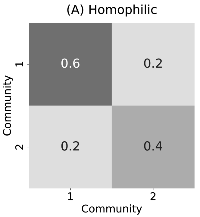
 
 
<center>![:scale 50%](images/honml/p1/homo_block_mtx.png)</center>

---

#### Block Models with PSD block matrices and RDPGs

If $\\mathbf A^{(1)}$ and $\\mathbf A^{(2)}$ are $IER_n(P)$ networks with probability matrices $P^{(1)}$ and $P^{(2)}$, we
call them .ye[stochastically equivalent] if $P^{(1)} = P^{(2)}$
- .ye[stochastically equivalent]: two random quantities are equal in terms of the parameters that govern them (for
$IER_n(P)$ networks, probability matrices)

---

#### Block Models with PSD block matrices and RDPGs

If $\\mathbf A^{(1)}$ and $\\mathbf A^{(2)}$ are $IER_n(P)$ networks with probability matrices $P^{(1)}$ and $P^{(2)}$, we
call them .ye[stochastically equivalent] if $P^{(1)} = P^{(2)}$

Recall that if [$B$ is PSD](#psd_bm), for a random network $\\mathbf A^{(1)} \\sim SBM_n(\\vec z, B)$ that:

SBM: $P^{(1)} = (C\\sqrt B)(C\\sqrt B)^\\top = XX^\\top$ where $X = C\\sqrt B$

RDPG: $\\mathbf A^{(2)} \\sim RDPG\_n(X)$ where $X = C\\sqrt B$
- $\\mathbf A^{(1)}$ (an SBM) is stochastically equivalent to $\\mathbf A^{(2)}$ (an RDPG)

--
- .ye[SBMs (and DCSBMs) with PSD block matrices are stochastically equivalent to some RDPG]

---

#### Stochastic equivalence of SBMs and RDPGs example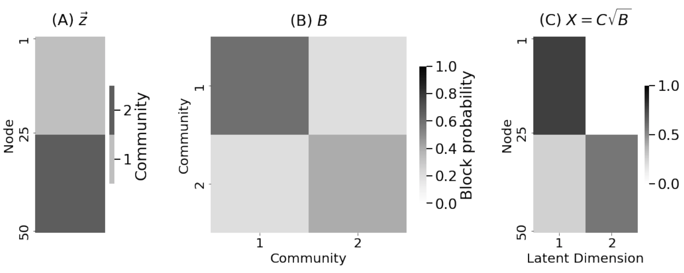

<center>![:scale 90%](images/honml/p1/psd_lpm.png)</center>

---

#### Stochastic equivalence of DCSBMs and RDPGs example

<center>![:scale 90%](images/honml/p1/psd_dcsbm.png)</center>

---

#### Block Models with PSD block matrices and RDPGs
- SBMs (and DCSBMs) with PSD block matrices are stochastically equivalent to some RDPG
- PSD matrices are very intuitive and easy to work with
- lots of linear algebra tricks and manipulations are designed for PSD matrices

---

#### Focus for second section

- develop techniques for RDPGs
- All techniques for RDPGs "work" for RDPGs and block models with PSD block matrices
- they work more generally with non PSD block matrices (advanced; unintuitive)

#### Key application
- the latent position matrix for RDPGs is tabular: $X$ is $n \\times d$
- Nodes are like "observations"
- latent dimensions of nodes are like "features"

---

### Coding example

See [Collab notebook](https://colab.research.google.com/drive/1CawEtJ9fdUNcKnIgq8o7ZQ-SSnZlVJWT?usp=sharing), Section 2

---
name:est

### Outline

- [Basics of Graph Data](#whyhave)
- [Random Graph Models](#models)
- Estimating Parameters for Networks
  - Estimating Network Representations
  - [Adjacency Spectral Embedding](#ase)
  - [Laplacian Spectral Embedding](#lse)
- [Applications](#apps)
- [Code example](#code)

### [Graph Neural Networks](#extra)

---

### Learning Representations of Networks

- Probability matrix $P$ tells us about structure of network

--
- But we never observe $P$! We observe adjacency matrices $A$

--
- So study "$\hat P$" from representations of $A$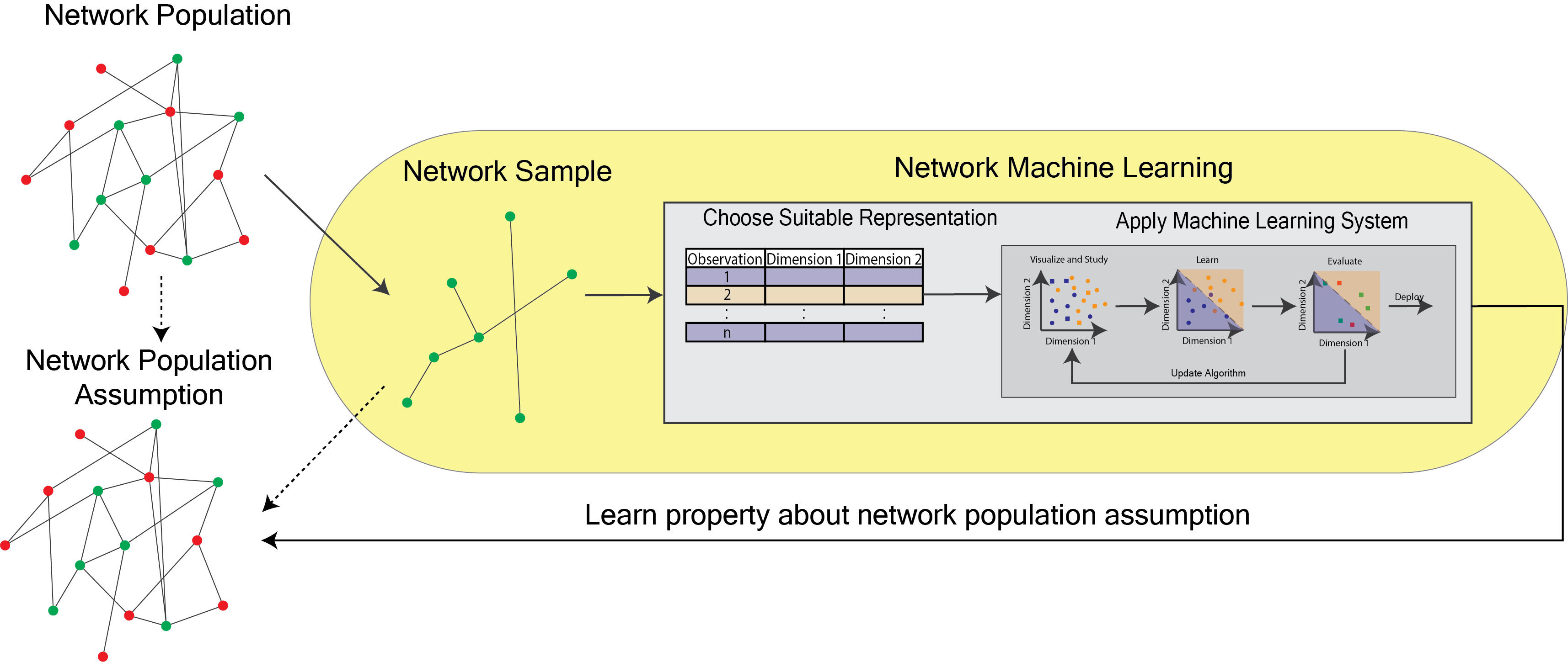

![:scale 100%](images/honml/p2/network_reps.png)

---
name:ase

### Outline

- [Basics of Graph Data](#whyhave)
- [Random Graph Models](#models)
- Estimating Parameters for Networks
  - [Network Representations](#est)
  - Adjacency Spectral Embedding
  - [Laplacian Spectral Embedding](#lse)
- [Applications](#apps)
- [Code example](#code)

### [Graph Neural Networks](#extra)

---

### Latent Positions from Probability Matrix

- Suppose we have a probability matrix $P$
    - Assume symmetric (undirected)

- If $P$ is PSD, then $P = XX^\\top$ with $X=\\sqrt P$.
    - Recall: PSD means you can take square roots.

- Assume $X$ has $n$ rows and $d$ columns
    - $n$ nodes, $d$ latent dimensions
    - none of the columns are redundant (the rank of $X$ is $d$).
    - entries are $\mathbb R$

- What does it mean to take a square root of a matrix?

---

### .ye[Eigendecomposition] ($\texttt{evd}$) of Symmetric Matrix

- Recall that if $R$ is a $n\times n$ symmetric matrix, then $R$ has an $\texttt{evd}$:

$$R = Q\Lambda Q^\top$$
- $\Lambda$: $n\times n$ diagonal matrix of the ordered (in decreasing order) eigenvalues of $R$
- $Q$: $n\times n$ matrix whose columns are eigenvectors of $R$.
- If $R$ is rank $d$, $\Lambda$ has $d$ non-zero eigenvalues; $n-d$ zero eigenvalues.

---

### $\texttt{evd}$ of Symmetric + PSD Matrix

- Assume $R$ is also PSD with rank $d$.
--

- Then $R$ has $d$ non-negative eigenvalues
  - $\lambda_1 \geq \lambda_2 \geq \cdots \geq \lambda_d > 0$
--

- With keeping $d$ non-zero eigenvalues
  - $Q_d$ : $n\times d$ matrix w/ first $d$ eigenvectors of $R$
  - $\Lambda_d$ : $d\times d$ diagonal matrix w/ first $d$ eigenvalues of $R$
  $$Q_d = \\begin{bmatrix}
  \\uparrow & & \\uparrow \\\\
  \\vec{q\_1} & ... & \\vec{q\_d} \\\\
  \\downarrow & & \\downarrow
  \\end{bmatrix},\Lambda_d = \\begin{bmatrix}
  \\lambda_1 & & \\\\
  & \ddots & \\\\
  & & \\lambda_d
  \\end{bmatrix}$$
- Decompose $R$ by
$$
R = Q_d\Lambda_d Q_d^\top
$$

---

### $\texttt{evd}$ of Probability Matrix $P$

- Let $P$ be $n\times n$ PSD matrix with rank $d$.

--
- We can obtain latent positions of $P$ by $\texttt{evd}$($P$)

$$
P = Q_d \Lambda_d Q_d^\top = (Q_d \sqrt{\Lambda_d})(Q_d \sqrt{\Lambda_d})^\top = XX^\top
$$

--
with

$$
X = Q_d \sqrt{\Lambda_d} = \sqrt{P}
$$

--
and

$$\sqrt{\Lambda_d} = \\begin{bmatrix}
\\sqrt\\lambda_1 & & \\\\
& \ddots & \\\\
& & \\sqrt\\lambda_d
\\end{bmatrix}$$
---

### Limitations of Eigendecomposition

- In practice, we never observe $P$, but observe the adjacency matrix $A$.
- So let's compute $\texttt{evd}$($A$)!

--
- If $A$ is PSD, then $\texttt{evd}$($A$) gives us _real_ latent positions of $A$.

--
- But what happens when $A$ is not PSD?
    - Can happen even if $P$ is PSD.

---

### Limitations of Eigendecomposition

- Consider the following probability and sampled adjacency matrix:

$$
P = \\begin{bmatrix}
0.5 & 0.5 \\\\
0.5 & 0.5
\\end{bmatrix},
A = \\begin{bmatrix}
0 & 1 \\\\
1 & 0
\\end{bmatrix}
$$

- $A$ is not PSD - it has eigenvalues $1$ and $-1$.
$$\Lambda = \\begin{bmatrix}
1 & \\\\
& -1
\\end{bmatrix}$$

--
- When we compute square root of $\Lambda$, we get a non-real matrix!
$$\sqrt\Lambda = \\begin{bmatrix}
1 & \\\\
& i
\\end{bmatrix}$$
--

$\implies$ results in non-real latent positions!

---

### .ye[Singular Value Decomposition] ($\texttt{svd}$) of Symmetric Matrices

- Recall that if $R$ is a $n\times n$ symmetric matrix, then $R$ has $\texttt{svd}$:
--
$$R = U \\Sigma V^\\top$$
- $\Sigma$ : $n\times n$ diagonal matrix of the ordered (in decreasing order) singular values of $R$
- $U$ : $n\times n$ the matrix whose columns are singular vectors of $R$.
    - Singular values are always real and non-negative
--
- If $R$ is rank $d$, $\Sigma$ has $d$ non-zero SVs; $n-d$ zero SVs
  - symmetry: if $R$ is symmetric and rank $d$, first $d$ columns of $V$ equal to first $d$ cols of $U$
--

- Taking the $d$ non-zero singular values:
$$R = U_d \\Sigma_d U_d^\\top$$

---

### $\texttt{svd}$ of Probability Matrix $P$

- Taking $\texttt{svd}$ of $P$:
$$
P = XX^\\top, X = U_d \\sqrt{\\Sigma_d}
$$

--
- Applying $\texttt{svd}$ to $A$ while keeping $d$ number of singular values/vectors:
$$\hat X = \hat U_d \sqrt{\hat \Sigma_d}$$
- Gives us an estimate of the probability matrix $P$.
$$\hat P = \hat X \hat X^\top$$
--

- This is called the .ye[adjacency spectral embedding].

---

### .ye[Adjacency] Spectral Embedding

- “Adjacency” - operates on the adjacency matrix $A$

---

### Adjacency .ye[Spectral] Embedding

- “Adjacency” - operates on the adjacency matrix $A$
- “Spectral” - intuition relies on the eigenvalues/eigenvectors

---

### Adjacency Spectral .ye[Embedding]

- “Adjacency” - operates on the adjacency matrix $A$
- “Spectral” - intuition relies on the eigenvalues/eigenvectors
- “Embedding” - finds a mathematical structure contained in another (a tabular structure contained within the adjacency matrix).

---

### Adjacency Spectral Embedding

##### Procedure

1. Decompose $A= U\\Sigma V^\\top$ via $\texttt{svd}$
2. Keep $d$ largest singular values, and obtain $U_d$ and $\Sigma_d$.
3. Compute $\sqrt{\Sigma_d}$ where entries are $\sqrt{\sigma_i}$ for $1,\ldots,d$.
4. Compute estimated latent positions $\hat X = U_d \sqrt{\Sigma_d}$.

---

### $\texttt{ase}$ Example - Sampling from SBMs

- Suppose we have SBM with $n = 100$ nodes and $K = 2$ communities.

---

### $\texttt{ase}$ Example - True vs Estimated Probability Matrices

<center>
 <img src="images/honml/p2/ase_result.png" style="background-color:white; width:80%" />
</center>
---

### $\texttt{ase}$ Example - Estimated Latent Positions

---

### Non-identifiability of RDPG

- .ye[Non-identifiability]: multiple solutions to the same problem
  - Many "reasonable" latent positions $X$ produce same $P$

--
- .ye[Rotational non-identifiability]: rotation of latent positions
- Given a rotation matrix $W$, and $Y=XW$:
    - RDPG$_n(X)$ and RDPG$_n(Y)$ have same probability matrix $P$
--
  - .ye[rotation matrix]: $WW^\\top = W^\\top W = I_d$
--

$$
\\begin{aligned}
P &= YY^\\top \\\\
&= XW(XW)^\\top \\\\
&= XWW^\\top X^\\top \\\\
&= XI_dX^\\top \\\\
&= XX^\\top
\\end{aligned}
$$

---

### Visualization of Rotational Non-identifiability

- Caveat: be careful when comparing different latent positions

---

### Why use $\texttt{ase}$ at all?

1. $\texttt{ase}$ tabularizes your adjacency matrix
  - $n\times d$ real matrix, where $d$ was the number of dimensions that you selected to embed into
  - explore the nodes using more traditional machine learning approaches

--
2. $\texttt{ase}$ decouples the dependencies of the random network
  - Want to study $P$ which encodes structure of networks
  - Let's study $X$ latent positions, which also encodes same structure

--
3. If we assume $\mathbf A$ is a random network,
  - theoretical results $\implies$ as our networks get larger (more data), our estimates of $P$ get better
  - $\hat X$ is a useful surrogate for studying $X$
  - can be useful even under model misspecification

---
name:lse

### Outline

- [Basics of Graph Data](#whyhave)
- [Random Graph Models](#models)
- Estimating Parameters for Networks
  - [Network Representations](#est)
  - [Adjacency Spectral Embedding](#ase)
  - Laplacian Spectral Embedding
- [Applications](#apps)

### [Graph Neural Networks](#extra)

---

### "Stretching" of latent positions in DCSBMs

- Recall: If $\\mathbf A \\sim DCSBM_n(\\vec z, \\vec \\theta, B)$, then if $B$ is PSD:
$$P = XX^\\top, X = \\Theta C \\sqrt{B}$$
  - the rows of $X$ can be written: $\\vec x\_i = \\theta\_i c\_{z_i} \\sqrt{B}$
--

- If $j$ is another node in the same community as $i$, note that $\\vec x\_j = \\frac{\\theta\_j}{\\theta\_i}\\vec x\_i$
  - .ye[all] nodes in community $z\_i$, this term is the same up-to the degree correction factor
--

- latent positions of DCSBMs are .ye[rescalings] of a shared latent position for each community (similar to SBM)
  - Consequence: latent positions are "stretched" along an axis

---

#### "Stretching" of latent positions in DCSBMs

- nodes in different communities are more similar (estimated lpm wise) than nodes in same community
<center>
 <img src="images/honml/p2/lse_ex.png" style="background-color:white; width:60%" />
</center>

---

### Laplacian Spectral Embedding ($\texttt{lse}$)

- Remember the [network Laplacian](#dad_lapl) is $L = D^{-\\frac{1}{2}} A D^{-\\frac{1}{2}}$
  - recall: entries are $l\_{ij} = \\frac{a\_{ij}}{\\sqrt{d\_i}\\sqrt{d\_j}}$

---

### Laplacian Spectral Embedding ($\texttt{lse}$)

- Remember the [network Laplacian](#dad_lapl) is $L = D^{-\\frac{1}{2}} A D^{-\\frac{1}{2}}$
  - recall: entries are $l\_{ij} = \\frac{a\_{ij}}{\\sqrt{d\_i}\\sqrt{d\_j}}$ .ye[these are normalized]
--

- .ye[Laplacian spectral embedding] is applying $\texttt{ase}$ to $L$
  - with $d$ number of latent dimensions:

$$L = \\hat X \\hat X^\\top, \\hat X = U_d \\sqrt{\\Sigma_d}$$

- Here, $\\hat X$ are the .ye[estimated latent positions of the network Laplacian]

---

### $\texttt{ase}$ vs $\texttt{lse}$

- Suppose $\\mathbf A$ is a DCSBM$_n(\\vec \\theta, \\vec z, B)$ random network with $n = 100$ nodes and $K = 2$ communities.

---

### $\texttt{ase}$ vs $\texttt{lse}$

- $\texttt{lse}$ preserves within-community structure with degree-corrections
- Intuitively makes sense since $L$ is normalized by node degree

---

### $\texttt{ase}$ vs $\texttt{lse}$

- How do we determine when to use $\texttt{lse}$?

--
- Tail heavy degree distributions

---

### Practical Considerations

- $d$ latent dimensions is a hyperparameter.

--
- How do we choose $d$?
 - Visual inspection of singular values (scree plot)
<center>
 <img src="images/honml/p2/Screeplotr.png" style="background-color:white; width:50%" />
</center>

--
    - Automated "elbow" detection algorithms
--
    - Try multiple $d$ and evaluate performance on subsequent tasks

---
name:apps

### Outline

- [Basics of Graph Data](#whyhave)
- [Random Graph Models](#models)
- [Estimating Parameters for Networks](#est)
- Applications
  - Community Detection
  - [Two-Sample Hypothesis Testing](#2samp)
- [Code example](#code)

### [Graph Neural Networks](#extra)

---

### What is community detection?

- Goal: find groups of nodes that are "similar" to each other than to all other nodes.

--
- Let's suppose you have a network $A$ with $n$ nodes.

--
    - Assume $\mathbf A\sim SBM_n$, but we don't know $\vec z$!
--
    - Community detection algorithms estimate $\vec z$.
--
- Note: In unsupervised learning, called clustering

##### Procedure for community detection
1. Learn representations of your network
  - Embed using $\texttt{ase}$ or $\texttt{lse}$ in $d$ dimensions
--

2. Cluster the representations
  - e.g. $K$-means
--

3. Evaluate your Clusters

---

### Example - Sampling from DCSBM

- Consider a DCSBM$_n$ with $n = 300$ nodes and $K = 3$ communities.
- Randomly shuffle the ordering of nodes.
--

- Can you find the communities?

---

### Example - Latent Positions from $\texttt{ase}$

- Estimate latent positions $\hat X$ from $\texttt{ase}$ of sampled adjacency matrix
- Label latent positions by apriori known communities

--
- $\hat X$ retains the community structure

---

### Estimate communities with 3-means

- Use 3-means clustering on $\hat X$
- Evaluate clustering by visualizing classification

---

### Clustering with Unknown Number of Communities

- In real data, number of communities are not obvious.
- How do we find "optimal" number of communities?

##### Procedure
1. Learn representations of your network
  - Embed using $\texttt{ase}$ or $\texttt{lse}$ in $d$ dimensions
--

2. For $k\in\{2, 3, \ldots, K\}$ number of communities
  1. Use k-means to cluster latent positions
  2. Compute .ye[silhouette score]
--

3. Choose $k$ that has the highest .ye[silhouette score]

---

### Example

---

### Practical Considerations

- Choice of embeddings
    - $\texttt{lse}$ can be robust to degree variations
    - Can even consider non-spectral embeddings!
        - node2vec
--
- Choice of embedding dimension $d$
    - Different $d$ can give different clustering results
--
- Choice of clustering algorithm
    - Gaussian mixture models ($\texttt{gmm}$) can give better results
    - Fuzzy clustering (soft clustering)

---

### [Two-Truths of Spectral Clustering](https://doi.org/10.1073/pnas.1814462116)

- Averaged from 100s human brain networks
  - Assume a 4-block SBM: {left, right} x {gray matter, white matter}
- Embed using $\texttt{ase}$ or $\texttt{lse}$
- Estimate 2 communities using $\texttt{gmm}$

---

### [Two-Truths of Spectral Clustering](https://doi.org/10.1073/pnas.1814462116)

| Clusters | $\texttt{gmm}$ o $\texttt{ase}$ | $\texttt{gmm}$ o $\texttt{lse}$|
| ---| --- | --- |
| 1 | right GM , left GM | right GM , right WM |
| 2 | right WM , left WM | left GM , left WM |

---

### [Two-Truths of Spectral Clustering](https://doi.org/10.1073/pnas.1814462116)

- Core-periphery: densely and sparsely connected within, densely connected across
- Affinity: densely connected within, sparsely connected across

---
name:2samp

### Outline

- [Basics of Graph Data](#whyhave)
- [Random Graph Models](#models)
- [Estimating Parameters for Networks](#est)
- Applications
  - [Community Detection](#apps)
  - Two-Sample Hypothesis Testing
- [Code example](#code)

### [Graph Neural Networks](#extra)

---

### What is Two-sample Hypothesis Testing?

- Given two networks $A^{(1)}$ and $A^{(2)}$:
--

- Are they the "same"? (null hypothesis $H_0$)
--

- Are they "different"? (alternate hypothesis $H_A$)
--

##### General Strategy
1. Assume a model for the networks
2. Formulate a hypothesis test based on the model
3. Compute a test statistic

##### Assumptions
  - Same number of nodes in both networks
  - One-to-one correspondence of nodes between both network

---

### Example - Traffic Patterns

- Goal: examine traffic pattern differences during the daytime (7AM-7PM) compared to night time (7PM-7AM).

--
- 100 towns (nodes) from $K=3$ states
  - 45 towns from NY
  - 30 towns from NJ
  - 25 towns from PA

--
- Measure the number of commuters from pairs of towns
  - If more than 1,000 drivers regularly make this commute, we add an edge between the pair of towns

--
- We have two networks:
  - the first network between 7 AM and 7 PM (covering the bulk of the work day)
  - the second network between 7 PM and 7 AM (covering the bulk of night time)

---

### Example - Traffic Patterns

---

### Testing Whether Block Matrices are Different

- Given block matrices $B^{(1)}$ and $B^{(2)}$

$$
B^{(1)} = \\begin{bmatrix}
b^{(1)}\_{11} & b^{(1)}\_{12} & b^{(1)}\_{13} \\\\
b^{(1)}\_{21} & b^{(1)}\_{22} & b^{(1)}\_{23} \\\\
b^{(1)}\_{31} & b^{(1)}\_{32} & b^{(1)}\_{33}
\\end{bmatrix},\;\;\; B^{(2)} = \\begin{bmatrix}
b^{(2)}\_{11} & b^{(2)}\_{12} & b^{(2)}\_{13} \\\\
b^{(2)}\_{21} & b^{(2)}\_{22} & b^{(2)}\_{23} \\\\
b^{(2)}\_{31} & b^{(2)}\_{32} & b^{(2)}\_{33}
\\end{bmatrix}
$$

--
- First hypothesis:
$$H_0: B^{(1)} = B^{(2)}; \ \ H_A: B^{(1)} \neq B^{(2)}$$

---

### Testing Whether Block Matrices are Different

- Given block matrices $B^{(1)}$ and $B^{(2)}$

- More concrete hypothesis:

$$H\_{0, kl}: b\_{kl}^{(1)} = b^{(2)}\_{kl}; \ \ H\_{A, kl} : b\_{kl}^{(1)} \neq b^{(2)}\_{kl}$$

--
- Statements about matrices to statement about probabilities

---

### Fischer's Exact Test

- For each $k$ and $l$ community pair, we can compute the $2\times 2$ contingency table:

|  | night time |  day time|
| ---| --- | --- |
| Number of edges | a | b |
| Number of non-edges | c  | d |

- Intuitively, tests whether proportion of edges is independent of time of day.

- Now we can compute the p-value for each $H\_{0, kl}$ hypothesis!

- What about multiple comparisons?

---

### Multiple Comparisons Problem

- Suppose we have 5000 fair coins (equal probability of heads and tails)
--

- For each coin
    - Flip the coin 500 times
--
    - Test $H_0^{(i)} : p^{(i)} = 0.5$ against $H_A^{(i)}: p^{(i)} \neq 0.5$
--
    - Compute the p-value of the hypothesis that the coin is fair

---

### Multiple Comparisons Problem

- .ye[Familywise error rate (FWER)]: probabiliy we incorrectly rejected the null

--
- Rescale p-values via .ye[Holm-Bonferroni] correction.
    - No assumptions on dependence of hypothesis tests

---

### Example - Traffic Patterns

- Hypothesis: $H\_{0, kl}: b\_{kl}^{(1)} = b^{(2)}\_{kl}; \ \ H\_{A, kl} : b\_{kl}^{(1)} \neq b^{(2)}\_{kl}$
--

- Take the minimum of the p-values for each $H\_{0, kl}$ hypothesis
  - If the minimum p-value is less than 0.05, reject the null hypothesis

- Reject the null hypothesis

---

### Testing If Block Matrices are Multiples of Each Other

- What if probability of edge was, in general, 50% higher during daytime?
    - Was previous result was just due to a scaling factor?
--
    - Want to find topolgical differences
--
- Modify previous hypothesis:
$$H_0: B^{(1)} = \alpha B^{(2)}; \ \ H_A: B^{(1)} \neq \alpha B^{(2)}$$
- We can take $\alpha$ to be the ratio $p^{(1)}/p^{(2)}$

---

### Example - Traffic Patterns

- Hypothesis: $H_0: B^{(1)} = \alpha B^{(2)}; \ \ H_A: B^{(1)} \neq \alpha B^{(2)}$
- Use chi-squared test

- Reject the null hypothesis
- After adjusting for differences in density, there exists differences in traffic patterns.

---

### Other interesting tests?

1. Are the latent positions from two networks different?

$$H_0: X = YW ;\ H_A: X \neq YW$$
--

2. Are the _distributions_ of latent positions from two networks different?

$$H_0: F_X = F_Y ;\ H_A: F_X \neq F_YW$$
--

3. Which latent positions are different from two networks?

$$H_0: X_i = Y_iW ;\ H_A: X_i \neq Y_iW$$

---

#### Focus for third section

- coding examples for network analysis

---

### Coding example

See [Collab notebook](https://colab.research.google.com/drive/1CawEtJ9fdUNcKnIgq8o7ZQ-SSnZlVJWT?usp=sharing), Section 3

---

name:extra

### Outline

- [Basics of Network Data](#whyhave)
- [Random Network Models](#models)
- [Estimating Parameters for Networks](#est)
- [Applications](#est)
- [Code example](#code)

### Graph Neural Networks
 - Random walks and "diffusion" on networks
 - [Skipgram network](#skip)

---

### Random walks and diffusion methods

- develop a stochastic process (random) that generates paths through the network
  - "random walk": paths generated from the stochastic process, but with repeats
  - "diffusion": start somewhere in the network, and end somewhere (randomly)

--
- diffusion methods on networks
  - do .ye[not] analyze the network itself

--
  - analyze the walks diffusing through the network

---

### Finite-space markov chains

- .ye[Finite-space markov chain]: random system where the possible events that can occur are finite
  - for network data, the "events" are visits to nodes in the network
  - If the network has $n$ nodes, the collection of possible events is $n$
- .ye[Random walk] for network data of length $T$: $(s\_0, \\mathbf s\_1, ..., \\mathbf s\_T)$
  - $\\mathbf s\_t$ is a node in the network (random)
  - $s\_0$ is termed the source node for the random walk, and is usually fixed
---

### First-order markov chains

- Random walk:  $(s_0, \\mathbf s\_1, ..., \\mathbf s\_T)$
  - $\\mathbf s\_1, ..., \\mathbf s\_T$ are determined through an evolutionary (random) process
- .ye[First-order markov chain]
  - Imagine that we have walked the sequence $(s\_0, ..., s\_t)$

--
$$\\mathbb P(\\mathbf s\_{t + 1} | s\_{t}, ..., s\_0) = \\mathbb P(\\mathbf s\_{t+1} | s\_{t})$$
- "The next node in the walk depends only on the current node that we are at"

---

### First-order markov chains with networks

- $p\_{ij} = \\begin{cases}\\frac{1}{d\_i},& a\_{ij} = 1 \\\\ 0, & a\_{ij} = 0\\end{cases}$
  - If we are at a node $i$ at step $t$, we choose the next node to visit in our walk randomly from the neighbors $j \in \mathcal N(i)$ of node $i$

--
  - $i$ has $d\_i$ neighbors, so each neighbor has an equal chance of being visited
- $p\_{ij}$: .ye[transition probability] from node $i$ to the next node $j$
  - does not depend on $t$; only on the current and next possible nodes

---

### Transition probability matrix

- $n \\times n$ matrix where the entries $p\_{ij}$ are the transition probabilities from $i$ to $j$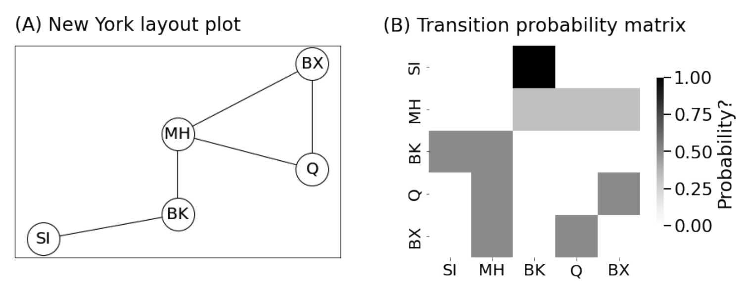

<center>![:scale 90%](images/honml/p1/tpm.png)</center>

---

### Transition example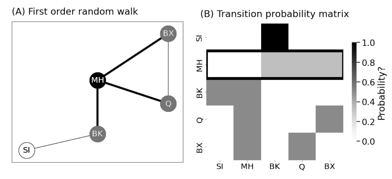

<center>![:scale 90%](images/honml/p1/trans_ex.png)</center>

---

### Obtaining a transition probability vector

- To actually implement a random walk programmatically, we need to return to matrices
- What we will do is use one-hot encodings of our current vectors
  - If $s\_{t} = i$, we will let $\\vec x^{(i)}$ be the vector where:

$$x\_j^{(i)} = \\begin{cases}1, & j = i \\\\ 0, & j \\neq i\\end{cases}$$

- If we are at MH, $\\vec x^{(MH)} = \\begin{bmatrix}0 & 1 & 0 & 0 & 0\\end{bmatrix}^{\\top}$
---

### Obtaining a transition probability vector

- We'll define the probability vector from node $i$ to be:

$$\\begin{aligned}
\\vec p\_i &= P^\\top \\vec x^{(i)} \\\\ 
&= \\begin{bmatrix} p\_{11} & \\cdots & p\_{1n} \\\\ \\vdots & \\ddots & \\vdots \\\\ p\_{n1} & \\cdots & p\_{nn}\\end{bmatrix}^{\\top}\\begin{bmatrix}x\_1^{(i)} \\\\ \\vdots \\\\ x\_n^{(i)}\\end{bmatrix} \\\\
&= \\begin{bmatrix} p\_{11} & \\cdots & p\_{n1} \\\\ \\vdots & \\ddots & \\vdots \\\\ p\_{1n} & \\cdots & p\_{nn}\\end{bmatrix}\\begin{bmatrix}x\_1^{(i)} \\\\ \\vdots \\\\ x\_n^{(i)}\\end{bmatrix}\\end{aligned}$$

---

### Obtaining a transition probability vector

Continuing, we get:

$$\\begin{aligned}
\\vec p\_i &= P^\\top \\vec x^{(i)} \\\\ 
&= \\begin{bmatrix}\\sum\_{i = 1}^n p\_{j1}x\_{j}^{(i)} \\\\ \\vdots \\\\ \\sum\_{i = 1}^n p\_{jn }x\_{j}^{(i)}\\end{bmatrix} \\\\
&= \\begin{bmatrix}p\_{i1} \\\\ \\vdots \\\\ p\_{in}\\end{bmatrix}
\\end{aligned}$$
because $x\_i^{(i)} = 1$ is the only entry that is non-zero (other sum terms drop out)
---
name:next_entry
##### The multinoulli distribution

$\\mathbf x \\sim \text{Multinoulli}(\\vec p)$ if:
1. $\\vec p$ is a probability vector ($\\sum\_{i = 1}^n p\_i = 1$)
2. $\\mathbf x$ has realizations $x \\in \\{1, \\cdots, n\\}$ (it is *categorical*)
3. $\\mathbb P(\\mathbb x = i) = p\_i$

##### Generating next entry of the random walk

Let $\\mathbf s\_{t + 1} \\sim \text{Multinoulli}(\\vec p\_{s\_t})$

---

### Algorithm for generating random walks

random_walk(P, s0):
    """
    P: the nxn transition probability matrix.
    s0: the source node.
    """
      Let s[0] = s0.
      For t from 1:T:
        Let x[i] = 1 where i = s[t - 1], and 0 otherwise.
        Let p = transpose(P)* x.
        Let s[t] be a Multinoulli sample with probability vector p.
      Return the random walk s.
    
---

name:skip

### Outline

- [Basics of Network Data](#whyhave)
- [Random Network Models](#models)
- [Estimating Parameters for Networks](#est)
- [Applications](#est)
- [Code example](#code)

### Graph Neural Networks
  - [Random walks and "diffusion" on networks](#extra)
  - Skipgram network
      
---

### Graph Neural Network Lexicon

- Note that we have two networks we are dealing with
1. The network: the object we are studying
2. The GNN: the network that we are using implicitly as part of the algorithm 
- We will be studying a technique called $\\texttt{DeepWalk}$

---

### Generating a "corpus" for our netework

- $\\texttt{DeepWalk}$ was designed from natural language processing techniques
  - most of the language around it uses NLP lingo
- .ye[corpus]: a collection of text (e.g., from a stack of documents) that we learn from
  - For $\\texttt{DeepWalk}$, we use random walks to construct a "corpus"

---

### Generating a "corpus" for our network

generate_corpus(T, R):
    """
    T: the walk length.
    R: the number of walks per node in the network.
    """
      For each source node i in 1:n:
        For each walk r in 1:R:
          Use the procedure developed to generate a random walk of length T,
          starting at node i.
      Return the collection of random walks.

---
### Skipgram GNN

- Idea: the random walks hold properties about the nodes
  - Nodes that tend to have lots of shared neighbors will tend to be "closer" on random walks, in general

--
- Dummy goal: given a node $i$, predict the probability that another node $j$ is $\\omega$-close to it
  - $\\omega$: the "window width"
  - If we can figure out nodes that tend to be "close" to a node $i$, perhaps we can use the GNN to extract information about the network

--
- Nodes that are are given are called .ye[center nodes]
  - Nodes that we want to predict are called .ye[context nodes]
  - "Context": under what contexts (nearby nodes) does our center node tend to show up?
---

### Using the corpus to produce training samples

- Center nodes: white
- Context nodes: gray
<center>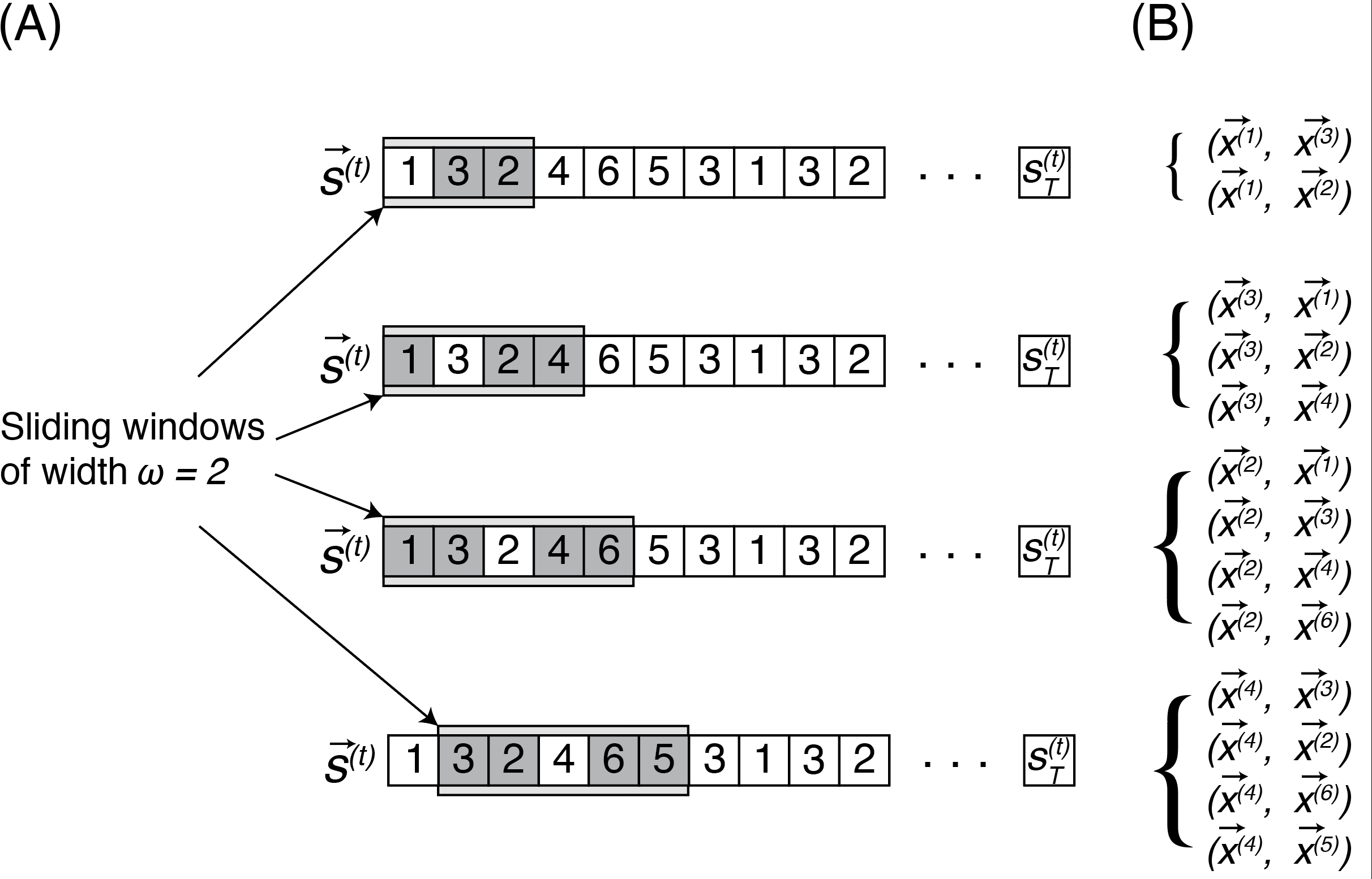![:scale 90%](images/honml/p1/skipgram_tr_samps.png)</center>

---

### The embedding process

- The GNN itself is extremely simple
  - Input layer: $n$ nodes (one for each node in the network)
  - Hidden layer: $d$ nodes
    - $d$: "embedding dimensions"
  - Output layer: $n$ nodes (one for each node in the network)

---

### Architecture of a skip-gram network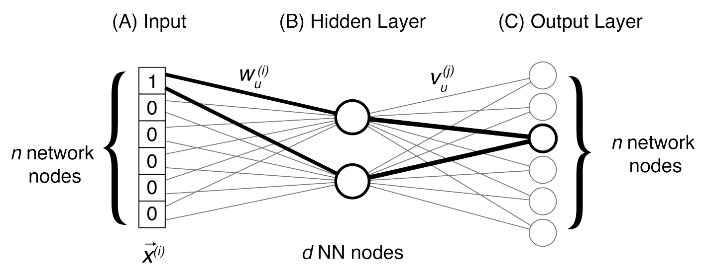

<center>![:scale 90%](images/honml/p1/skipgram_arch.png)</center>

---

### The embedding layer

- To connect the input layer to the hidden nodes, we have an "embedding layer"
  - The "embedding layer" describes a weight matrix $W$ which is $n \\times d$
  - $\\vec x^{(i)}$ is $n$-dimensional
$$W = \\begin{bmatrix} \\leftarrow & \\vec w^{(1)\\top} & \\rightarrow \\\\ & \\vdots & \\\\ \\leftarrow & \\vec w^{(n)\\top} & \\rightarrow \\end{bmatrix}$$

---

### The embedding matrix

- To connect the input layer to the hidden nodes, we have an "embedding matrix"
- We take the product $W^\\top \\vec x^{(i)}$ to be the "embedding" of the node $i$
  - Since $W^\\top$ is $d \\times n$ dimensions and $\\vec x^{(i)}$ is an $n$-vector, the product is $d$-dimensional
$$W^\\top = \\begin{bmatrix} \\uparrow & & \\uparrow \\\\ \\vec w^{(1)} & \\cdots & \\vec w^{(n)} \\\\ \\downarrow & & \\downarrow\\end{bmatrix}$$

---

### The embedding process

$$\\begin{aligned}W^\\top \\vec x^{(i)} &= \\begin{bmatrix} \\uparrow & & \\uparrow \\\\ \\vec w^{(1)} & \\cdots & \\vec w^{(n)} \\\\ \\downarrow & & \\downarrow\\end{bmatrix}
\\begin{bmatrix}x^{(i)}\_1 \\\\ \\vdots \\\\ x^{(i)}\_n\\end{bmatrix} \\\\
&= \\begin{bmatrix}\\sum\_{j = 1}^n w^{(j)}\_1 x\_j^{(i)} \\\\ \\vdots \\\\ \\sum\_{j = 1}^n w^{(j)}\_d x\_j^{(i)}\\end{bmatrix}\\end{aligned}$$
- Remember: $x\_j^{(i)} = 1$ only when $j = i$, and is zero otherwise (one-hot encoding)
---

### The embedding process

$$\\begin{aligned}W^\\top \\vec x^{(i)} &= \\begin{bmatrix}\\sum\_{j = 1}^n w^{(j)}\_1 x\_j^{(i)} \\\\ \\vdots \\\\ \\sum\_{j = 1}^n w^{(j)}\_d x\_j^{(i)}\\end{bmatrix}\\\\
&= \\begin{bmatrix}w^{(i)}\_1 \\\\ \\vdots \\\\ w^{(i)}\_{d}\\end{bmatrix} = \\vec w^{(i)}\\end{aligned}$$

- The "embedding" of $x^{(i)}$ really just extracts the $i^{th}$ row of $W$
---

### The "softmax" function

- When are are trying to predict probabilities, a typical choice is the "softmax" function
- If you have done logistic regression, you have used this before
- The .ye[softmax] for an $n$-element vector $\\vec y$ is the $n$-element vector with entries:

$$\\sigma(\\vec y)\_j = \\begin{bmatrix}\frac{\\exp(y\_j)}{\\sum\_{j' = 1}^n \\exp(y\_{j'})}\\end{bmatrix}$$

- Note that the exponential is strictly positive (for non-infinite $y\_j$), so the numerator is strictly less than the denominator
- By construction, $\\sum\_{j = 1}^n \\sigma(\\vec y)\_j = 1$
  - it produces probabilities
---

### The "projection" matrix provides predicted probabilities

- The first step in the projection layer is to use another matrix $V$ to "project" the embedding back to a $d$-dimensional vector
  - We do this by taking the product $V^\\top \\vec w^{(i)}$
  - $V$ is a $d \\times n$ matrix, and $\\vec w^{(i)}$ is a $d$-vector, so we obtain a $n$-vector
- We then apply the softmax to the result, and the predicted probability for context node $j$ with center node $i$ is:
$$p^{(i)}\_j(W, V) = \\sigma\\big(V^{\\top} \\vec w^{(i)}\\big)\_j$$

---

### A forwards pass through a Skipgram network

- To conclude off the description of the Skipgram network, we will use something known as a loss function
- The loss function is the cross-entropy loss, which for a single training sample $\\big(\\vec x^{(i)}, \\vec x^{(j)}\\big)$:
$$L\_{i,j}(W, V) = \\vec x^{(j)} \\log\\bigg(\\vec p^{(i)}(W, V)\\bigg)$$

---

### Forwards pass through a Skipgram network (schematic view)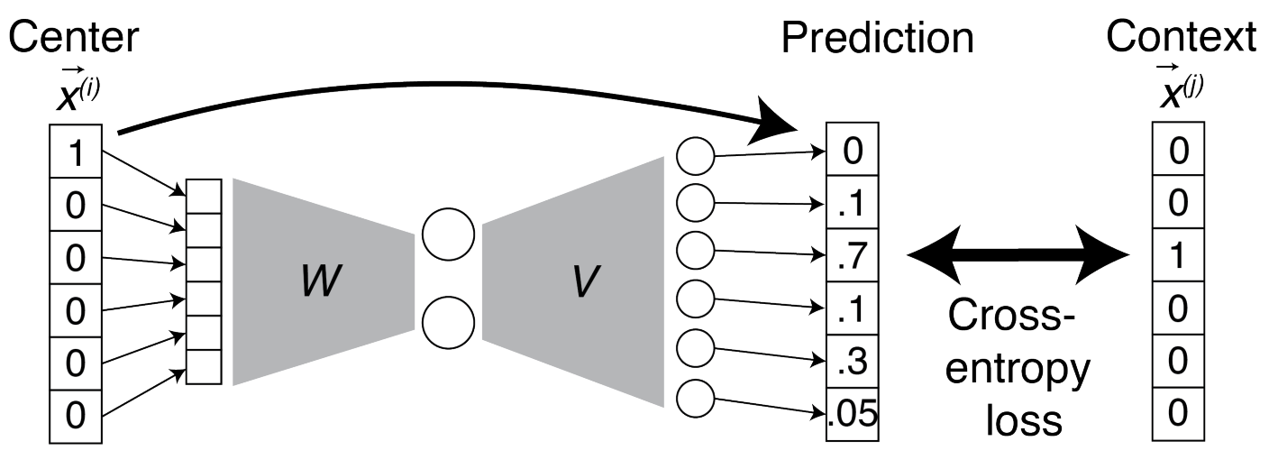

<center>![:scale 90%](images/honml/p1/skipgram_schem.png)</center>

---

### How do we actually train the Skipgram network?
1. Randomly reorder the training data into "epochs" which contain one instance of every training sample (in random order).

--
2. Split the epochs into $B$ batches.

--
3. For each batch:
  - Run a forwards pass for every training sample in that batch, and compute the cross-entropy loss.
  - Compute the cumulative loss as the sum of the cross-entropy losses for each training sample in the batch.
  - Use backpropogation to update the embedding matrix $W$ and the projection matrix $V$.

--
4. Repeat for all epochs, until arbitrary stopping criterion is met.

--
5. Use the rows $\\vec w^{(i)}$ as the embedding for node $i$.

---

### Skip-gram networks in action

- What we described is known as $\\texttt{DeepWalk}$
  - it uses first-order random walks
- There are many other diffusion-based GNNs that use other types of random walks
  - $\\texttt{node2vec}$: second-order biased random walks

---

### Skip-gram networks in action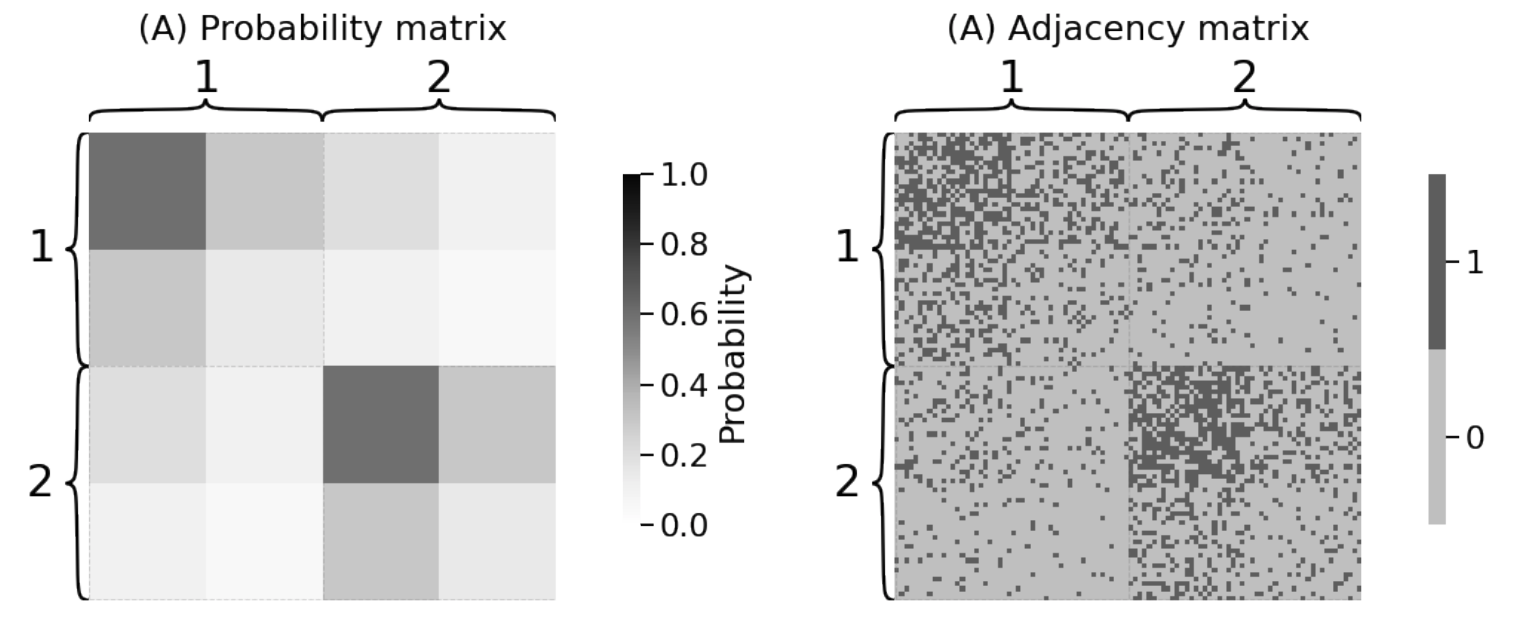

<center>![:scale 90%](images/honml/p1/skipgram_ex.png)</center>

- 2 homophilic communities, and each community has nodes with high degrees (core) and low degrees (periphery)

--
  - DCSBM??

---

### Skip-gram networks in action

<center>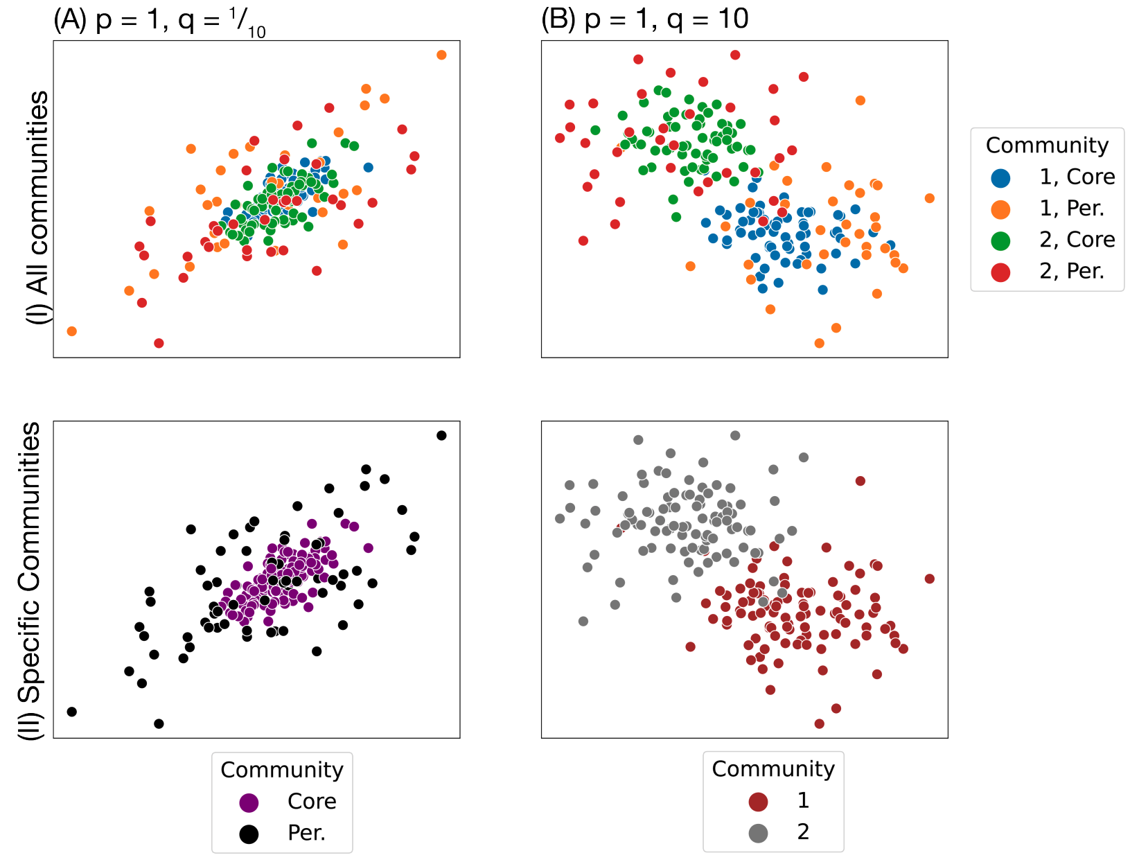![:scale 90%](images/honml/p1/skipgram_result.png)</center>